Establishing Norms for the Robustness of Automatic Speech Recognition
From CNBH Acoustic Scale Wiki
Roy D. Patterson, Jessica Monaghan, Christian Feldbauer, Martin D. Vestergaard and Thomas C. Walters
The overall purpose of this research project is to develop a practical auditory preprocessor for automatic speech recognition (ASR) that adapts to glottal-pulse rate (GPR) and normalizes for vocal tract length (VTL) without the aid of context and without the need for training. The auditory preprocessor would make ASR much more robust in noisy environments, and more efficient in all environments. The first phase of the research involved constructing a version of the auditory image model (AIM) for use at AFRL/IFEC with documentation illustrating how the user can perform GPR and VTL normalization. The current report describes the development of performance criteria, or ‘norms’, for the robustness of automatic speech recognition (ASR) – norms that can also be used to compare with the robustness of human speech recognition (HSR). A companion report describes the development of comparable norms for the robustness of HSR using traditional psychophysical methods. The development of the ASR norms employed Mel Frequency Cepstral Coefficients (MFCCs) as features and Hidden Markov Models (HMMs) for the training and recognition. The results show that this traditional ASR system is much less robust to changes in vocal tract length than HSR, as was predicted. The ASR test is valuable in its own right inasmuch as it can be run on prototype systems as they are developed to assess their inherent robustness, relative to the traditional ASR recognizer, and to track improvements in robustness as ASR performance converges towards HSR performance.
The text and figures on this page are from a project report associated with an EOARD grant (FA8655-05-1-3043) entitled Measuring and Enhancing the Robustness of Automatic Speech Recognition
Roy Patterson , Jessica Monaghan , Tom Walters
Contents |
INTRODUCTION
When a child and an adult say the same word, it is only the message that is the same. The child has a shorter vocal tract and lighter vocal cords, and as a result, the waveform carrying the message is quite different for the child. The fact that we hear the same message shows that the auditory system has some method for ‘normalizing’ speech sounds for both Glottal Pulse Rate (GPR) and Vocal Tract Length (VTL). These normalization mechanisms are crucial for extracting the message from the sound that carries it from speaker to listener. They also appear to extract specific VTL and GPR values from syllable-sized segments of an utterance as it proceeds. In noisy environments with multiple speakers, the brain may well use these streams of GPR and VTL values to track the target speaker and so reduce confusion. Current speech recognition systems use spectrographic preprocessors that preclude time-domain normalization like that in the auditory system, and this could be one of the main reasons why ASR is so much less robust than Human Speech Recognition (HSR) in multi-source environments (MSEs). To wit, Potamianos et al. (1997) have shown that a standard speech-recognition system (hidden Markov model) trained on the speech of adults, has great difficulty understanding the speech of children. This new perspective, in which GPR and VTL processing are viewed as preliminary normalization processes, was made possible by recent developments in time-scale analysis (Cohen, 1993), and the development of an auditory model (Irino and Patterson, 2002) showing how Auditory Frequency Analysis (AFA) and auditory GPR normalization could be combined with VTL normalization to extract the message of the syllable from the carrier sound.
The overall purpose of this research project is to develop a practical auditory preprocessor for ASR systems – a preprocessor that performs GPR and VTL normalization without the aid of context and without the need for training. The auditory preprocessor would make ASR much more robust in noisy environments, and more efficient in all environments. The first phase of the research involved constructing a version of AIM for use at AFRL/IFEC with documentation illustrating how the user can perform GPR and VTL normalization. The current report describes the development of performance criteria, or ‘norms,’ for the robustness of automatic speech recognition (ASR) – norms that can also be used to compare the robustness of ASR and HSR. The results show that ASR is not robust to variation in VTL when trained on the speech of speakers with only a small range of VTLs. The robustness improves if the speech sounds in the training data are scaled using STRAIGHT to increase the range of GPRs and VTLs in the training data – a technique that may well be applicable to training data in general. A companion report describes the development of comparable norms for the robustness of human speech recognition (HSR) using traditional psychophysical techniques. The final section of the report compares the robustness data obtain from the ASR and HSR, and is common to the two reports. The remainder of this introduction describes the internal structure of speech sounds and the concept of normalization as it pertains to speech sounds.
The internal structure of speech Sounds


At the heart of each syllable of speech is a vowel; Figure 1 shows four versions of the vowel /a/ as in ‘hard’. From the auditory perspective, a vowel is a ‘pulse-resonance’ sound, that is, a stream of glottal pulses each with a resonance showing how the vocal tract responded to that pulse. Many animal calls are pulse resonance sounds. From the speech perspective, the vowel contains three important components of the information in the larger communication. For the vowels in Fig. 1, the ‘message’ is that the vocal tract is currently in the shape that the brain associates with the phoneme /a/. This message is contained in the shape of the resonance which is the same in every cycle of all four waves. In the left column, one person has spoken two versions of /a/ using high (a) and low (b) GPRs; the pulse rate (PR) determines the pitch of the voice. The resonances are identical since it is the same person speaking the same vowel. In the right-hand column, a small person (c) and a large person (d) have spoken versions of /a/ on the same pitch. The pulse rate and the shape of the resonance are the same, but the rate at which the resonance proceeds within the glottal cycle is slower in the lower panel. This person has the longer vocal tract and so their resonance rings longer. VTL is highly correlated with the height of the speaker (Fitch and Giedd, 1999). In summary, GPR corresponds to the pitch of the voice, the shape of the resonance corresponds to the message, and resonance rate corresponds to VTL and, thus, to speaker size.
Normalization of speech sounds
The essence of GPR and VTL normalization is illustrated in Fig. 2; it shows how the information in the vowel sound, /a/, can be segregated and used to construct a ‘pulse image’ and a ‘resonance image’, each with their own time-difference dimension, Δtp and Δtr. The scale is logarithmic in both cases. The upper panel shows the neural activity produced by the /a/ sound of Fig. 1 in the auditory filter centred on the second formant of the vowel (near 1500 Hz). The largest peaks in the wave are from the glottal pulses; they bound the resonances in time and control the pulse normalization process. It is assumed that when the neural representation of glottal pulse, pn, reaches the brainstem, it initiates a pulse process and a resonance process both of which run until the next glottal pulse arrives. The pulse process simply waits for the next pulse, and when it arrives, calculates the time difference, (Δtp=tn+1-tn) and increments the corresponding bin by the height of the pulse. The pulse, pn+1, terminates the pn process and initiates a new pulse process, and so on. The image decays continuously in time with a half life of about 30 ms, so when the period of the wave is 10 ms or more, the peak in the image is essentially stable because it is incremented three or more times in the time it would take to decay to half its height. This is the essence of Pulse-Rate Normalization (PRN). The resonance process is very similar to the pulse process; however, during the time between pulses, it adds a copy of the resonance behind the current pulse, into the resonance image. So the resonance values in the image are each incremented by the value of the resonance at t – tn. The half life of the resonance image is the same as the pulse image. Now consider the pulse and resonance images that would be produced by the waves in Figure 1. The wave in (a) would produce a stable peak at 6 ms in the pulse image and a stabilized version of the resonance in the resonance image. When the glottal period increases to 12 ms as in (b), the peak at 6 ms in the pulse image would decay away over about 100 ms as a new peak rises at 12 ms. The resonance in the region 0 < Δtr < 6 would not change. When the resonance expands as in (d), the peak in the pulse image at Δtp = 8 ms would be unaffected. The resonance function would shift a little to the left (larger Δtr values) without changing shape. This is the essence of Resonance Scale Normalization (RSN). The resonance shape is the message; the distance from the origin represents the length of the vocal tract. These processes can be applied to all of the channels of AFA to produce the complete analysis of the syllable. In summary, these simple normalization processes segregate the GPR information from the VTL information, and segregate the resonance scale information from the resonance shape information (the message).
METHODS, ASSUMPTIONS AND PROCEDURES
The overall purpose of the current study is to develop a paradigm for research on the robustness of ASR (Allen, 2005) including a means of comparing the robustness of ASR with the robustness of HSR. This section of the report describes the development of norms for the robustness of ASR; the corresponding section of the companion report described the development of norms for the robustness of HSR. The two studies employed the same set of stimuli – a structured database of simple syllables and the same response measure – ‘percent correct syllable recognition’. The main difference between the HSR and ASR studies is in the training and the systems used to perform the recognition, that is, the human brain verses a computer-based, HMM recognizer using MFCC features.
Structured, syllable corpus
A structured corpus of simple syllables was used to establish both the ASR robustness norms and the HSR robustness norms. The corpus was compiled by Ives et al. (2005) who used phrases of four syllables to investigate VTL discrimination and show that the just-noticeable difference (JND) in speaker size is about 5 %. There were 180 syllables in total, composed of 90 pairs of consonant-vowel (CV) and vowel-consonant (VC) syllables, such as ‘ma’ and ‘am’. There were three consonant-vowel (CV) groups and three vowel-consonant (VC) groups as shown in Table I. Within the CV and VC categories, the three groups were distinguished by consonant category: sonorants, stops, or fricatives. So, the corpus is a balanced set of simple syllables in CV-VC pairs, rather than a representative sample of syllables from the English language. The vowels were pronounced as they are in most five vowel languages, like Japanese and Spanish, so that they could be used with a wide range of listeners. A useful mnemonic for the pronunciation is the names of the notes of the diatonic scale, “do, re, mi, fa, so” with “tofu” for the /u/. For the VC syllables involving sonorant consonants (e.g., oy), the two phonemes were pronounced separately rather than as a diphthong.

The syllables were recorded from one speaker (author RP) in a quiet room with a Shure SM58-LCE microphone. The microphone was held approximately 5 cm from the lips to ensure a high signal to noise ratio and to minimize the effect of reverberation. A high-quality PC sound card (Sound Blaster Audigy II, Creative Labs) was used with 16-bit quantization and a sampling frequency of 48 kHz. The syllables were normalized by setting the RMS value in the region of the vowel to a common value so that they were all perceived to have about the same loudness. We also wanted to ensure that, when any combination of the syllables was played in a sequence, they would be perceived to proceed at a regular pace; an irregular sequence of syllables causes an unwanted distraction. Accordingly, the positions of the syllables within their files were adjusted so that their perceptual-centers (P-centers) all occurred at the same time relative to file onset. The algorithm for finding the P-centers was based on procedures described by Marcus (1981) and Scott (1993), and it focuses on vowel onsets. Vowel onset time was taken to be the time at which the syllable first rises to 50 % of its maximum value over the frequency range of 300-3000 Hz. To optimize the estimation of vowel onset time, the syllable was filtered with a gammatone filterbank (Patterson et al., 1992) having thirty channels spaced quasi-logarithmically over the frequency range of 300-3000 Hz. The thirty channels were sorted in descending order based on their maximum output value and the ten highest were selected. The Hilbert envelope was calculated for these ten channels and, for each, the time at which the level first rose to 50 % of the maximum was determined; the vowel onset time was taken to be the mean of these ten time values. The P-centre was determined from the vowel onset time and the duration of the signal as described by Marcus (1981). The P-center adjustment was achieved by the simple expedient of inserting silence before and/or after the sound. After P-center correction the length of each syllable, including the silence, was 683 ms.
Scaling the syllable corpus
Once the syllable recordings were edited and standardized, a vocoder referred to as STRAIGHT (Kawahara and Irino, 2005) was used to generate all the different ‘speakers,’ that is, versions of the corpus in which each syllable was transformed to have a specific combination of VTL and GPR. STRAIGHT uses the classical source-filter theory of speech Dudley (1939) to segregate GPR information from the spectral-envelope information associated with the shape and length of the vocal tract. STRAIGHT produces a pitch-independent spectral envelope that accurately tracks the motion of the vocal tract throughout the syllable. Subsequently, the syllable can be resynthesized with arbitrary changes in GPR and VTL; so for example, the syllable of a man can be readily transformed to sound like a women or a child. The vocal characteristics of the original speaker, other than GPR and VTL, are preserved by STRAIGHT in the scaled syllable. Syllables can also be scaled well beyond the normal range of GPR and VTL values encountered in everyday speech and still be recognizable (e.g., Smith et al., 2005). The central speaker in both the HSR and ASR studies was assigned GPR and VTL values on the line between the average adult man and adult woman on the GPR-VTL plane, and mid-way between the adult man and woman, where both the GPR and VTL dimensions are logarithmic. Peterson and Barney (1952) reported that the average GPR of men is 132 Hz, while that of women is 223 Hz, and Fitch and Giedd (1999) reported that the average VTLs of men and women were 155.4 and 138.8 mm, respectively. Accordingly, the central speaker was assigned a GPR of 171.7 Hz and a VTL of 146.9 mm. For scaling purposes, the VTL of the original speaker was taken to be 165 mm.

The important variable in both the ASR and the HSR experiments is the distance along a spoke from the reference voice at the center of the spoke pattern to a given test speaker. The distance is referred to as the Radial Scale Distance (RSD). It is the geometrical distance from the reference voice to the test voice, which is
 where X and Y are the coordinates of GPR and VTL, respectively, in this log-log-space, and χ is the GPR-VTL trading value, 1.5. The speaker values were positioned along each spoke in logarithmically increasing steps on these logarithmic co-ordinates. The seven RSD values were 0.0071, 0.0283, 0.0637, 0.1132, 0.1768, 0.2546, and 0.3466. There are eight speakers associated with each RSD value, and their coordinates form ellipses in the logGPR-logVTL plane. The seven ellipses are numbered from one to seven, beginning with the innermost ellipse, with an RSD value of 0.0071.
| Spoke | Point: | 1 | 2 | 3 | 4 | 5 | 6 | 7 |
| 1 | GPR (Hz) | 170.9 | 168.6 | 164.7 | 159.5 | 153.0 | 145.5 | 137.0 |
| VTL (cm) | 14.7 | 14.8 | 14.9 | 15.1 | 15.3 | 15.5 | 15.8 | |
| 2 | GPR (Hz) | 171.3 | 170.0 | 167.8 | 164.9 | 161.1 | 156.7 | 151.6 |
| VTL (cm) | 14.8 | 15.0 | 15.5 | 16.2 | 17.0 | 18.2 | 19.7 | |
| 3 | GPR (Hz) | 171.9 | 172.4 | 173.3 | 174.5 | 176.1 | 178.1 | 180.4 |
| VTL (cm) | 14.8 | 15.1 | 15.6 | 16.4 | 17.5 | 18.8 | 20.6 | |
| 4 | GPR (Hz) | 172.4 | 174.5 | 178.0 | 183.0 | 189.6 | 198.1 | 208.6 |
| VTL (cm) | 14.7 | 14.9 | 15.2 | 15.6 | 16.2 | 16.8 | 17.7 | |
| 5 | GPR (Hz) | 172.5 | 174.9 | 179.0 | 184.8 | 192.7 | 202.7 | 215.2 |
| VTL (cm) | 14.7 | 14.6 | 14.5 | 14.3 | 14.1 | 13.9 | 13.6 | |
| 6 | GPR (Hz) | 172.1 | 173.5 | 175.7 | 178.8 | 183.0 | 188.1 | 194.5 |
| VTL (cm) | 14.6 | 14.3 | 13.9 | 13.4 | 12.7 | 11.9 | 11.0 | |
| 7 | GPR (Hz) | 171.5 | 171.0 | 170.1 | 168.9 | 167.4 | 165.6 | 163.4 |
| VTL (cm) | 14.6 | 14.3 | 13.8 | 13.2 | 12.4 | 11.5 | 10.5 | |
| 8 | GPR (Hz) | 171.0 | 169.0 | 165.7 | 161.1 | 155.5 | 148.8 | 141.3 |
| VTL (cm) | 14.6 | 14.5 | 14.2 | 13.8 | 13.4 | 12.8 | 12.2 |
Table II: GPR and VTL values for the scaled speakers.
In the ASR study, the HMM recognizer was trained on the data from one of three different ellipses: numbers one, four and seven with RSD values of 0.0071, 0.1132, and 0.3466, respectively. In each case, the recogniser was tested on the remaining speakers. The HMM recogniser was initially trained on the reference speaker and the voices of ellipse number one, that is, the eight speakers closest to the reference speaker in the GPR-VTL plane. This initial experiment was intended to imitate the training of a standard, speaker-specific ASR system, which is trained on a number of utterances from a single speaker. The eight adjacent points provided the small degree of variability needed to produce a stable hidden Markov model for each syllable. The recogniser was then tested on all of the scaled speakers, excluding those used in training, to provide an indication of the native robustness of the ASR system. The elliptical distribution of speakers, across the GPR-VTL plane, was chosen to reveal how performance falls off as GPR and VTL diverged from those of the central speaker. Statistical learning machines do not generalize well beyond their training data. Thus, it was not surprising to find that the performance of the speaker-dependent recogniser was not robust; performance falls off rapidly as VTL diverges from that of the reference speaker. Statistical learning machines are rather better at interpolating, rather than extrapolating, and so the recogniser was retrained, first with the speakers on ellipse four, and then with the speakers on ellipse seven, to see if giving the system experience with a larger range of speakers would enable it to interpolate within the ellipse and so improve performance. The eight points in ellipses four and seven were used as the training sets in these two experiments. The results are presented in the next section.
In the HSR study, pilot testing made it clear that performance would be good throughout the GPR-VTL plane, and as a result, the listeners were only trained with the central, reference speaker and then tested with the speakers on ellipse seven with the RSD value, 0.3466. These are the speakers at the ends of the spokes with GPR and VTL values most different from the reference speaker. A comparison of the ASR and HSR results is presented in the final section of the Results and Discussion section below.
Mel-Frequency, Cepstral Coefficients as features for ASR
A Mel-Frequency, Cepstral Coefficient (MFCC) is the amplitude of a cosine function fitted to a spectral frame of a sound (plotted in quasi-log-frequency, log-magnitude coordinates). The calculation involves four steps. First a temporal window is applied to the sound and a fast Fourier transform is performed on this windowed signal. Then, the spectrum is mapped onto a Mel-frequency scale using a triangular filter-bank, and spectral magnitude is converted to log-magnitude. The mel-frequency scale is a quasi-logarithmic scale, similar to the ERB scale used in AIM, and it is used to map human pitch perception on to a linear scale. Finally, a Discrete Cosine Transform (DCT) is performed on the ‘mel-frequency, magnitude spectrum’. The MFCCs are the coefficients of the cosine series expansion. All coefficients above the thirteenth are discarded which has the effect of smoothing the spectral envelope. The process removes the spectral fine structure including most of the information about harmonic spacing (i.e., the pitch of the voice). The zero coefficient of the MFCC series is proportional to the log of the energy of the sound. The windowing used to produce the MFCCs does not preserve the pulse resonance structure of sound. There is a software package referred to as the HMM tool kit (HTK) (Young et al., 2006) which can be used to create Hidden Markov Models based on MFCC vectors for ASR. The essentials are described below. HTK provides a tool, Hcopy, which takes a list of files in .wav format with their parameters and calculates a sequence of MFCC vectors for the sounds in the files. In the current study, Hcopy was used to create a sequence of MFCC vectors for each of our syllables in all of its forms. The temporal window was a Hamming function with a duration of 25ms; the frame step was 10ms. The mel-frequency filterbank had 26 channels, that is, there were 26 points on the mel-frequency spectrum. These were the default settings. Matlab scripts were used to index the .wav files in the database for use by Hcopy. The input to the recognizer included the 13-coefficient vectors provided by Hcopy, supplemented by first difference vectors between pairs of MFCC vectors (referred to as delta vectors), and second difference vectors between pairs of delta vectors (acceleration vectors referred to as delta-delta vectors). A long series of studies that this combination of MFCC vectors provides a reasonable summary of the information in speech sounds for studying ASR.

4. A three state, Hidden-Markov Model for syllable recognition
The Hidden-Markov-model Toolkit (HTK) was used to create a three state, hidden Markov model for syllable recognition, using feature vectors composed of 13 MFCCs. HTK models speech as a sequence of stationary segments, or frames, produced by a Markov model (e.g., Figure 5). The Markov model has non-emitting initial and final states and an indefinite number of emitting states between them. The probability of moving between one state, i, and the next state, j, as a function of time, is given by a discrete probability, aij. Only transitions forward in time from left to right are permitted. As the states are passed through in time steps, they emit a series of equally spaced feature vectors characteristic of the sound being produced. These feature vectors are assumed to give an accurate representation of a frame of speech, which is typically of the order of 10ms. The probability of a state, i, emitting a feature vector, ot, is given by a probability density, bi(ot). The initial and final non-emitting states are used to produce the composite model used in continuous speech recognition. They are used to indicate the probability of a given syllable being followed or preceded by another syllable, and so they are not used in isolated syllable recognition.
If a syllable is modelled as a sequence of feature vectors, O = o1, o2, ... oT, the recognition problem is solved by finding the i that maximizes P(si|O), where si is the ith syllable. Using Bayes’s theorem this probability is:
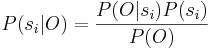 , so for a given set of priors P(si) the probability depends only on the likelihood P(O|si). For isolated word recognition the priors for each syllable will be equal. P(O) is a normalisation term which is the same for all syllables and so can be ignored. The generative model of speech assumes that P(O|si) = P(O|Mi), where Mi is the Markov model corresponding to the syllable si. This is useful because it replaces the problem of measuring the observation probability density P(O|si), which has a high dimensionality, with the simpler problem of estimating the parameters of the hidden Markov model which can be done with training.
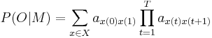
In a hidden Markov model, the state sequence X, the transition probabilities, and the output probabilities are unknown and must be inferred from the training data, O. Given a set of training examples corresponding to a particular syllable model, the parameters of that model can be determined automatically by a robust and efficient iterative clustering procedure. The task of recognition is to find a maximum value for the probability of obtaining the observed sequence of feature vectors from a particular HMM:
, so for a given set of priors P(si) the probability depends only on the likelihood P(O|si). For isolated word recognition the priors for each syllable will be equal. P(O) is a normalisation term which is the same for all syllables and so can be ignored. The generative model of speech assumes that P(O|si) = P(O|Mi), where Mi is the Markov model corresponding to the syllable si. This is useful because it replaces the problem of measuring the observation probability density P(O|si), which has a high dimensionality, with the simpler problem of estimating the parameters of the hidden Markov model which can be done with training.
In a hidden Markov model, the state sequence X, the transition probabilities, and the output probabilities are unknown and must be inferred from the training data, O. Given a set of training examples corresponding to a particular syllable model, the parameters of that model can be determined automatically by a robust and efficient iterative clustering procedure. The task of recognition is to find a maximum value for the probability of obtaining the observed sequence of feature vectors from a particular HMM:
 , over all models M.
This is approximated by considering only the most probable state sequence:
, over all models M.
This is approximated by considering only the most probable state sequence:
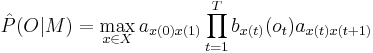 Although it is not possible to calculate this directly, HTK is able to compute it efficiently using an iterative Viterbi algorithm.
Training the HMM with HTK
In HTK, HMM definition files consist of the transition probabilities aij , stored in a transition matrix, and output probability densities, bi, defined by a vector of means and a covariance matrix. The probability density of each syllable HMM is assumed to be a multi-variate Gaussian distribution over the components of the feature vectors. The multi-variate Gaussian distribution is a generalisation, to higher dimensions, of the one dimensional Gaussian distribution, and it is given by:
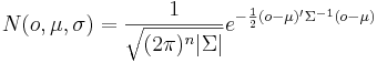 ,where Σ is the covariance matrix of the feature vectors, μ is a vector of the means, and o is the feature vector. Initially, a prototype definition is used to describe the topology of the HMM, and the actual numbers used in the definition are not important. The transitions allowed between states are indicated by putting non-zero values in the corresponding elements of the transition matrix and zeros elsewhere. For the prototype, the vector size and parameter type (e.g. MFCC) must be specified, as well as the number of states of the model. The prototype model is initialised by the user and re-estimated by HTK. In general, the components of the feature vectors are assumed to be independent and a diagonal covariance matrix is used.
Initially, the HMM used for the MFCC recogniser had three emitting states, which is sufficient for the duration of a single syllable; the output distributions were simply Gaussian. Subsequently, the topology of the HMM was improved by changing the number of states and introducing Gaussian mixture models into the output distributions. The number of states and Gaussian mixtures were later varied to maximise the recognition rate.
Training begins with the tool HcompV, which takes as its input the prototype HMM, which indicates the probability distribution to be used, and a list of training data. It then initialises the HMM for each syllable to be identical and to have state means and variances equal to the global speech mean and variance of the training data. Training data consists of one or more examples of each utterance, in the form of frames of feature vectors, together with a transcription (label) file to assign each example to the correct HMM.
,where Σ is the covariance matrix of the feature vectors, μ is a vector of the means, and o is the feature vector. Initially, a prototype definition is used to describe the topology of the HMM, and the actual numbers used in the definition are not important. The transitions allowed between states are indicated by putting non-zero values in the corresponding elements of the transition matrix and zeros elsewhere. For the prototype, the vector size and parameter type (e.g. MFCC) must be specified, as well as the number of states of the model. The prototype model is initialised by the user and re-estimated by HTK. In general, the components of the feature vectors are assumed to be independent and a diagonal covariance matrix is used.
Initially, the HMM used for the MFCC recogniser had three emitting states, which is sufficient for the duration of a single syllable; the output distributions were simply Gaussian. Subsequently, the topology of the HMM was improved by changing the number of states and introducing Gaussian mixture models into the output distributions. The number of states and Gaussian mixtures were later varied to maximise the recognition rate.
Training begins with the tool HcompV, which takes as its input the prototype HMM, which indicates the probability distribution to be used, and a list of training data. It then initialises the HMM for each syllable to be identical and to have state means and variances equal to the global speech mean and variance of the training data. Training data consists of one or more examples of each utterance, in the form of frames of feature vectors, together with a transcription (label) file to assign each example to the correct HMM.

A program was written in Matlab to train the HMMs (see Figure 6). It produced the prototype HMM definition file and a list of training data files to be passed on to HCompV. HCompV produced an initial estimate HMM where the means and variances of each state were set equal to global means and variances of the training data. This estimate was then duplicated for each of the syllables to produce an HMM definition file. This set up is termed a ‘flat start’. Label files were produced for all the files, containing a transcript of their contents. HERest was called with the HMM definition and label files. HERest performs one Baum-Welch re-estimation each time it is called, training each syllable model only on training data labelled as that syllable. It produces a re-estimated HMM definition file as its output. It was used eight more times to produce well trained HMMs.
4.2 The recognition stage
HTK provides a recognition tool called HVite which performs Viterbi-based speech recognition. HVite takes, as input, a network describing the allowable word sequences, a dictionary, a set of HMM definitions, and a list of the files on which recognition is to be performed. For an isolated syllable recogniser the network indicates that the file will contain one of a given list of syllables preceded and followed by silence. The dictionary in this case is a list of the syllables. HVite gives a transcription of each file as its output. The Viterbi algorithm finds the state sequence that has the highest probability of occurring while generating the observation sequence, i.e., the maximum of the joint probability of the observation sequence and the state sequence, maxXP(X,O|M). The recognition process selects the maximum of found by the Viterbi algorithm over all models, and the syllable corresponding to that model is given in an output transcription file.
A second program was written to test the data on the remainder of the database (see Figure 7). For each of the test files HVite produces a transcription, as determined by its maximum likelihood procedure. The tool HResults computes the accuracy of the recognition performed by HVite by comparing the transcriptions produced with label files created for the test file. As well as recognition statistics, it produces a list of the misidentified files together with their labels and their incorrect transcriptions. A Matlab script was used to interpret the error transcription file produced by HResults and to compute and plot what percentage of the 185 syllables were correctly identified for each value of GPR and VTL.
RESULTS AND DISCUSSION
The results of the HSR experiment
The HMM recogniser was initially trained on the reference speaker and the voices of ellipse number one, with RSD value, 0.0071, that is, the eight speakers closest to the reference speaker in the GPR-VTL plane. This initial experiment was intended to imitate the training of a standard, speaker-specific ASR system, which would be trained on a number of utterances from a single speaker. The eight speakers immediately adjacent to the reference speaker provided the small degree of variability needed to produce a stable hidden Markov model for each syllable. The recogniser was then tested on all of the scaled speakers, excluding those used in training, to provide an indication of the native robustness of the ASR system. This initial experiment used an HMM topology with three emitting states and a single Gaussian output distribution for each state. The average performance for the recognizer was only 65.0 percent correct.
The distribution of performance across speakers is shown in Fig. 8. There is a central region adjacent to the training data for which performance is 100 %; it includes the second ellipse of speakers and several speakers along spokes 1 and 5 where VTL does not vary much from that of the reference speaker. As VTL varies further from the training values, performance degrades rapidly. This is particularly apparent in spokes three and seven, where recognition falls close to 0% for the extremes, and to a lesser extent in spokes two, four, six and eight. This demonstrates that this MFCC recogniser cannot extrapolate beyond its training data to speakers with different VTL values. In contrast, performance remains consistently high along spokes 1 and 5, where the main variation is in GPR. This is not surprising since the process of extracting MFCCs eliminates most of the GPR information from the features.
There is no straightforward optimisation technique for HMM topology. To ensure that the results were representative of HMM performance, a number of different topologies were trained and test. Performance was maximised for a HMM topology consisting of four emitting states, with several Gaussian mixtures making up the output distributions for each emitting state. The number of training stages was also varied to avoid over-training. The optimum recognition rate using the best topology was 73.5% after nine iterations of the training algorithm HERest. In the second test, the HMM recognizer was trained on the eight speakers of the fourth ellipse (RSD = 0.1132), and then it was tested on all of the remaining points in the database. The average recognition rate rose from 65% to 90.5%. The distribution of performance across speakers is shown in Fig. 9. Performance in the central region within the fourth ellipse is almost 100 % correct; performance has also improved along spokes 4 and 8 in the region beyond the fourth ellipse. It is only the extremities of spokes 2, 3, 6, and 7 where the VTL difference is large that performance falls off. The fact that performance improved substantially with this new training set (which had one less speaker) demonstrates that it is not the small size of the training set that caused the poor recognition results in the initial test. Rather it is a demonstration of the finding that HMM recognizers of this sort cannot extrapolate beyond the data set – a common finding with statistical learning machines.

In the final test, the HMM recognizer was trained on the eight speakers of the seventh ellipse (RSD = 0.3466), and then it was tested on all of the remaining points in the database. The average recognition rate rose immediately from 90.5% to 98.64%, and variation of the topology revealed performance levels as high as 99.85%. The distribution of performance across speakers is shown in Fig. 10 for completeness; performance is universally high across the GPR and VTL plane, even at the centre of the plane where no training data were provided.
Taken together, the results from the three experiments provide a dramatic demonstration of the fact that HMM/MFCC recognisers can interpolate but not they cannot extrapolate. That is, they cannot generalize from one speaker (or a set of very similar speakers) to speakers with different VTLs; but they can generalize from a disperse set of speakers to members within the space covered by the set. The training sets for the initial and final tests were essentially the same size, and the range of the extrapolation required in the first test is, in some sense, the same as the range of interpolation required in the final test; but the latter training strategy is clearly much more successful.
Comparison of the HSR and ASR robustness results
The robustness of HSR to variability in VTL stands in marked contrast to the lack of robustness for the speaker-specific ASR system trained on the reference speaker and speakers on the ellipse with the smallest RSD, 0.0071. The human listeners had previous experience with speakers whose GPR and VTL values vary from that of the reference speaker in the direction along spoke 1 where there are speakers similar to men of various sizes, and in the direction of the wedge between spokes 5 and 6 where there are speakers similar to women and children in the normal population. So it is not surprising that they performed well with these speakers. However, speakers with combinations of GPR and VTL like those in the wedges between spokes 6 and 8, and between spokes 2 and 4 become novel rapidly as RSD increases, and human performance was just as good with almost all of these speakers. The data support the view of Irino and Patterson (2002) that the auditory system has mechanisms that adapt to the GPR of the voice and normalize for acoustic scale prior to the commencement of speech recognition. Speech scientists are not surprised by listeners’ ability to understand speakers with unusual combinations of GPR and VTL, presumably because they have considerable experience of their own normalization mechanisms. The interesting point in this regard is that they often over generalize when it comes to statistical learning machines and predict that they too will be able to generalize and readily understand speakers with unusual combinations of GPR and VTL.

The results from the ASR study show that there is a marked asymmetry in the performance of HMM/MFCC recognizers between extrapolation and interpolation. When the recognizer was trained on speakers with only a small range of GPR and VTL combinations, it had great difficulty extrapolating to speakers with different VTLs. This result is important because this is precisely the way most commercial recognizers are trained, that is, on the voice of a single person. If the person is an adult member, the recognizer is very unlikely to work for a child, and vice verse. Fortunately, the study suggests a solution to the VTL aspect of the robustness problem: When the recognizer was trained on speakers with a wide range of combinations of GPR and VTL, its robustness improved dramatically. This suggests that the speech sounds used to train a machine recognizer should be scaled with STRAIGHT, or some other pitch-synchronous scaling algorithm, to simulate speakers with a wide range of combinations of GPR and VTL.
CONCLUSIONS
A syllable recognition task was developed to establish norms for the robustness of HSR and ASR – norms that could be used to monitor the robustness of an ASR system during development and track its improve towards the performance that might be expected from human listeners. HSR performance on the syllable task was found to be highly robust to variation in both GPR and VTL. The performance of a standard HMM/MFCC recognizer on the syllable task was not robust to variation in VTL when it was trained on a group of speakers having only a small range of VTLs. When it was trained on a group of speakers having a wide range of VTLs, robustness improved dramatically. The results suggests that the speech sounds used to train a machine recognizer should be scaled with STRAIGHT, or some other pitch-synchronous scaling algorithm, before training so that the training set simulates speakers with a wide range of combinations of GPR and VTL.
Acknowledgements
The research was supported by the UK Medical Research Council (G0500221; G9900369) and by the Air Force Office of Scientific Research, Air Force Material Command, USAF, under grant number FA8655-05-1-3043. The U.S. Government is authorized to reproduce and distribute reprints for Government purpose notwithstanding any copyright notation thereon. The views and conclusions contained herein are those of the author and should not be interpreted as necessarily representing the official policies or endorsements, either expressed or implied, of the Air Force Office of Scientific Research or the U.S. Government.
References
Allen, J.B. (2005). Articulation and intelligibility. In D. Pisoni, R. Remez (Eds.), Handbook of speech perception. Blackwell: Oxford UK
Cohen, L. (1993). The scale transform. IEEE Trans. ASSP, 41, 3275-3292.
Dudley, H. (1939). Remaking speech, Journal of the Acoustical Society of America, 11, 169-177.
Fitch, W.T., Giedd, J. (1999) Morphology and development of the human vocal tract: a study using magnetic resonance imaging. Journal of the Acoustical Society of America, 106, 1511-1522.
Irino, T., Patterson, R.D. (2002). Segregating Information about Size and Shape of the Vocal Tract using the Stabilised Wavelet-Mellin Transform, Speech Communication, 36, 181-203.
Kawahara, H., Irino, T. (2005). Underlying principles of a high-quality, speech manipulation system STRAIGHT, and its application to speech segregation. In P. Divenyi (Ed.), Speech separation by humans and machines. Kluwer Academic: Massachusetts, 167-179.
Marcus, S. M. (1981). Acoustic determinants of perceptual center (p-center) location. Perception and Psychophysics, 52, 691-704.
Patterson, R.D., Holdsworth, J. and Allerhand M. (1992). Auditory Models as preprocessors for speech recognition. In: M. E. H. Schouten (ed), The Auditory Processing of Speech: From the auditory periphery to words. Mouton de Gruyter, Berlin, 67-83.
Peterson, G.E., Barney, H.L. (1952). Control methods used in a study of the vowels. Journal of the Acoustical Society of America, 24, 175-184.
Scott, S. K. (1993). P-centres in Speech: An Acoustic Analysis. Doctoral dissertation, University College London.
Smith, D.R.R., Patterson, R.D., Turner, R., Kawahara, H., Irino, T. (2005). The processing and perception of size information in speech sounds. Journal of the Acoustical Society of America, 117, 305-318.
Young, S., Evermann, G., Gales, M., Hain, T., Kershaw, D., Liu, X., Moore, G., Odell, J., Ollason, D., Povey, D., Valtchev,V., Woodland, P. (2006). The HTK Book (for HTK version 3.4). Cambridge University Engineering Department, Cambridge.