Auditory-Based Processing of Communication Sounds/Features from the Auditory Image

From CNBH Acoustic Scale Wiki

Thomas C. Walters

In chapter 2 of this thesis, I took an observed property of the human auditory system -- that it is capable of correctly recognising pulse-resonance sounds which have had their resonance scale modified to well beyond the normal range of experience -- as the inspiration for a scale-shift invariant feature representation. The features were tested using a database of syllables which had been scaled to simulate speakers with a range of vocal tract lengths and glottal pulse rates. In chapter 3, I focused on the properties of strobed temporal integration, a mechanism whereby the auditory system might generate a stabilized representation of the neural patterns coming from the cochlea. In this chapter the feature representation developed in chapter 2 and the stabilised auditory images generated by strobed temporal integration are combined to create a feature representation which we hypothesise should have the scale-invariance properties of the original features and the noise-robustness properties of the stabilised auditory image. The various feature variants are compared with each other and with the standard MFCC features used in chapter 2.

The stabilised auditory image

The auditory image model (AIM) (Patterson et al., 1995) provides a framework for creating a stabilized auditory image (SAI) from the output of a filterbank. This representation of the signal is stable for sounds which are perceived by listeners as being stable. Theoretically, it is also more noise-robust than a simple filterbank representation (Patterson et al., 1992; Patterson, 1994), since the strobed temporal integration process causes the neural patterns associated with successive cycles of a periodic sound to reinforce each other in the SAI.

The stabilised auditory image (SAI) is a two-dimensional representation of an input sound. A single SAI is a snapshot of the audio in a short window around a point in time. The SAI changes continuously with time, and successive snapshots can be concatenated to make a movie of these two-dimensional frames. The first dimension of an SAI frame is simply the spectral dimension added by the filterbank. The second dimension comes from the strobed temporal integration process by which an SAI is generated. Strobed temporal integration works by locating prominent peaks, or 'strobes', in the incoming signal and calculating 'lags' relative to these times. These peaks are most commonly associated with the pulses in pulse-resonance sounds, for example the glottal pulses in speech. When a strobe occurs in a channel, a short segment of the signal following the peak in that channel is added to a buffer, starting at zero lag. The signals following multiple strobe points add constructively in the buffer. This process leads to a stable spectro-temporal representation of the microstructure in the signal following each pulse in the input sound.

The SAI was introduced in chapter 1, and the process by which strobe points can be detected was discussed at length in chapter 3. In this chapter, features generated from SAI-based representations are developed and tested. A useful property of the SAI is that it is stable when the input sound is perceived as being stable. Temporal averaging is performed in a 'smart' way - such that there is no 'beating' between the windowing function and the pulse rate of the incoming signal (Kawahara and Irino, 2004). The strobed temporal integration process also makes the representation of pulse-resonance sounds robust to interfering noise; pulse-resonance sounds will tend to be accentuated in this representation, since the strobed temporal integration process will lead to multiple pulses and resonances being placed on top of one another in the SAI, causing them to interfere constructively. By contrast, noises which have no temporal regularity will not be reinforced in this way, and will appear at a lower level relative to the pulse-resonance sounds since they will not, in general, interfere constructively.

In this section, the noise-robustness of the SAI is tested, using the syllable-recognition task described in chapter 2. Instead of generating features from the NAP, AIM-C was used to generate a SAI, which was then transformed into a size-shape image (SSI). To generate features for use in a recognition system, various spectral profiles of this image are computed and used as the input for the Gaussian fitting scheme described in chapter 2.

SAI marginals

Figure 1 -- An SAI with its temporal and spectral profiles

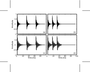
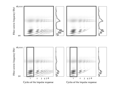
To a first approximation, it is possible to summarise the SAI by its marginals -- that is the vectors describing the mean of the SAI along its horizontal and vertical dimensions. These marginals are known as the `temporal profile' and `spectral profile' of the image. The SAI spectral profile is essentially a smoothed and temporally averaged version of the filterbank output. The temporal profile summarises information concerning the time intervals between prominent NAP pulses, and the time intervals in the fine structure following prominent pulses. Figure 1 shows an SAI, together with its temporal and spectral profiles.

Undersampling

Having said that the SAI segregates the pulse rate information and the resonances, it is still the case that changes in the pulse rate must have an effect on the structure of the resonances in the signal. This effect is easy to see by considering a pulse-resonance signal in the frequency domain. In this domain, a single damped resonance corresponds to some continuous frequency distribution. An idealised pulse train will have a frequency spectrum that also looks like a pulse train, with all harmonics of the pulse rate present in the spectrum. The pulse-resonance generation model has a stream of pulses exciting resonances of the vocal tract or other body. The time-domain pulse train and resonance are convolved to give the pulse resonance signal. This corresponds to a multiplication of the resonance envelope by a comb of peaks in the frequency domain: the resonance is `sampled' at the harmonics of the driving function. Thus although the pulse-resonance production mechanism allows a signal to be generated over longer time scales than the length of a single damped resonance, in doing so it causes information about the structure of the resonance to be lost. At higher pulse rates, the spectrum is sampled more sparsely, and so more information is lost. This `undersampling problem' is described in detail by de Cheveigné and Kawahara (1999).

The SSI

The 'scale-shift covariant' or 'size-shape' image (SSI) is another two-dimensional frame-based representation of the audio signal. It is obtained from a transformation of the SAI, and is a VTL covariant representation of the input signal. This means that changes in VTL correspond to simple shifts of the image. Patterson et al. (2007) provide an overview of the mathematics of the SSI and the process of generating images.

Figure 2 --- Four synthetic two-formant vowels, that differ in pitch and VTL. The upper two vowels (a) and (b) are for a short VTL with low and high GPR respectively. The lower two vowels (c) and (d) are for the same two GPRs with a longer VTL. This figure was prepared by Ralph van Dinther in connection with Patterson et al. (2007). Used with permission.

Figure 3 --- Idealised SSIs for one cycle of four synthetic two-formant vowels, as shown in Figure 2. This figure was redrawn from a figure by Ralph van Dinther. Used with permission.

The SSI is calculated from the SAI by taking the signal in each channel, and truncating it to leave the portion between zero-lag and the first peak associated with the next excitation pulse, that is the peak that completes the pitch period. This peak can be found in most cases by looking for the next highest peak in the SAI channel after the peak at zero-lag. Each of these truncated signals is then plotted as a function of cycles of the impulse response for the filter in that particular channel. In practice, this means that the time axis of each channel in the SAI is independently dilated by an amount proportional to the centre frequency of the filter in that channel. This has the effect of lining up the cycles of the impulse response of the filters. Interestingly, this transformation also has the effect of normalising out the faster decay rate of higher-frequency resonances in pulse-resonance sounds. This means that for a simple VTL change, because the auditory filterbank introduces a quasi-logarithmic scale on the vertical axis of the SSI, the pattern of formants in the SSI will shift as a unit up and down the vertical (cochlear place) axis of the image. With a logarithmic horizontal 'cycles' axis as well, the truncation of the signal at the pitch period of the incoming waveform has the effect of placing a diagonal `cutoff line' in the SSI at the point where the next pitch period begins. As pitch changes, this cutoff line retains the same gradient, but shifts its position up and down the image.

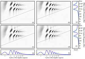
Figure 3 shows idealised SSIs for the four vowels in Figure 2. The SSIs are `idealised' in the sense that they are generated from a single cycle of the source vowel. The blue diagonal line in each case shows the cutoff line where the next pitch period would begin. In panel (d) where the source vowel has a high pitch and is from a long vocal tract, the pitch cutoff line clearly interferes strongly with the formant pattern. This is another manifestation of the undersampling problem.

Figure 4 --- SSI for a real human /a/ vowel.

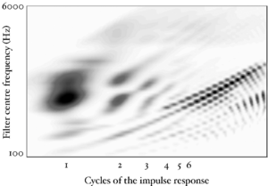
Figure 4 shows an SSI for a real human /a/ vowel. The pitch cutoff line is clearly visible as a strong diagonal in the image. Beyond this line, subsequent cycles of the waveform are squashed into a smaller and smaller space. The useful information in such an image is all in the area to the left and above the pitch cutoff line.

If it is possible to do accurate pitch detection in the SAI, then the SSI can be truncated at the pitch-cutoff line as it is generated. Accurate pitch detection is straightforward for single-source problems, however for images that contain multiple independent sources, the problem becomes more challenging.

The form of the information in the SSI

Figure 5 --- The form of the information in the SSI.

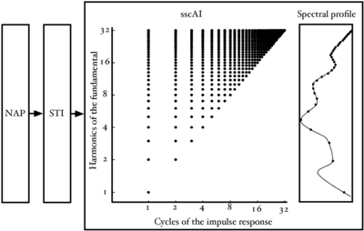
Figure 5 shows the points in the SSI where the information in pulse-resonance sounds is concentrated. Channel centre frequency is along the vertical dimension and time interval along the horizontal dimension. The units in the vertical dimension are harmonics of the fundamental. The units in the horizontal dimension are cycles of the impulse response.

In the frequency dimension, the points of interest are dictated by the pulse rate of the waveform. We have seen previously that for a pulse-resonance sound with a nonzero pulse rate, the spectral envelope will be sampled at the harmonics of the pulse rate. These harmonics are logarithmically spaced on the ERB axis of the auditory filterbank. This leads to the logarithmic spacing of points in the frequency dimension. In the time-interval dimension, the main points of interest are the peaks of the cycles of the impulse response in each channel. The response of the filter can be approximated by the amplitudes of the time domain peaks.

Dimensionality reduction

The transforms that convert a sound into an auditory image are intended to project the incoming signal into a space where pulse-resonance sounds are enhanced relative to background noise, and changes in acoustic scale leave the pattern of information largely unchanged, save for a spatial shift. While noise robustness and scale invariance are attractive properties, the transforms used to construct the space produce an explosion in the data rate which is a serious problem for an engineer trying to develop a speech recognizer. Whereas the data rate of the original sound is on the order of 300kbps, the data rate of the auditory image is on the order of 30Mbps. There are clearly substantial redundancies in the SAI and it behoves us to try and find a compact vector of features that summarises the signal and reduces the data-rate burden, if the SAI is to be used as the basis of a recognition system.

Chapter 6 details a method of producing a compact summary of features from the output of AIM-like models, and compares them to MFCCs, the traditional features in automatic speech recognition and sound classification. In the remainder of this chapter, the Gaussian features developed in chapter 2 are used to summarise spectral slices of the SSI, and the robustness of these features to noise is compared with that of the MFCCs and the features derived from the NAP in chapter 2.

Profiles and slices of the size-shape image

The SSI can be generated either with or without the pitch cut-off line. In the case of an SSI without the pitch cutoff, the second and subsequent pitch periods are `squashed' together in the lower right corner of the image. To generate the pitch cutoff for the experimental features described below, the temporal profile of the SAI was taken and the largest peak after the zero-lag peak is taken as the most prominent pitch period in the signal. There is a short `lockout' period of 4.6ms after the zero-lag peak, during which peak detection is suppressed, to allow the temporal profile to decay sufficiently. This allows detection of pitches up to around 217Hz. This allows for coverage of all pitches in the syllable database used for training and testing. However, more generally, spoken pitches may exceed this value and so the system would need to be modified to include a more robust pitch tracker in order to use the truncated SSI for features.

For both the full SSI and the truncated SSI, features were generated in two different ways. In each case, a spectral profile was constructed from the SSI and this was used with the Gaussian fitting procedure introduced in chapter 2. In the first variant, the spectral profile of the complete SSI was taken and used for fitting. In the second variant, a vertical `slice' of the SSI around the peak of the first cycle of the impulse response was taken, and the spectral profile of just this slice was taken.

In the case of the pitch-truncated SSI, for higher pitches, the lower-frequency regions of both these profiles may be zeroed-out. This can lead to a discontinuity in the spectral profile at that point. No attempt was made to smooth out this discontinuity before passing the profile to the Gaussian fitting procedure.

Figure 6 shows the regions of the SSI used to calculate the four feature variants used in the experiments, and the spectral profile for each region.

Figure 6 --- The four SSI variants used in the experiments. Each SSI is for the same /i/ vowel, spoken by a male. The left-hand SSIs are without the pitch cutoff, the right-hand SSIs are with the pitch cutoff. The grey boxes denote the region which is included in the spectral profile calculation. Spectral profiles for the region in the grey box are plotted to the right of each SSI. The large boxes cover the whole image, the small boxes just cover the first cycle of the filter impulse response in each channel.

Experiments

Comparison with features from the NAP

Recognition performance with these new SSI-based features was compared with that of the NAP-based features of chapter 2, using the syllable recognition task of chapter 2. The NAP features were compared with each of the four feature variants derived from the SSI. In these initial experiments, there was no noise background.

For each of the variants, the spectral profiles of successive image frames were fitted using the Gaussian fitting procedure described in chapter 2. This generates a 4-dimensional feature vector, containing the three relative weights of the Gaussians and a total energy term, as before. Delta, and delta-delta coefficients were calculated from these features, and the complete 12-dimensional feature vector was passed to the HMM recognition system described in chapter 2.

Figure 7 --- Scaled syllable recognition performance on the full SSI profile with no pitch cutoff.

Figure 8 --- Scaled syllable recognition performance on the full SSI profile with the pitch cutoff.

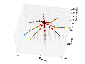
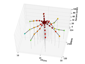
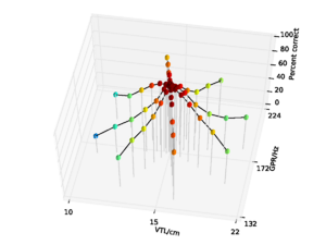
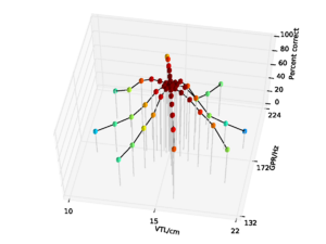
Figure 7 shows the performance of the whole-SSI features with no pitch cutoff on the syllable database. Performance is 84.8% overall, falling to a low of 31.6% at the shortest VTL. Figure 8 shows the performance for the SSI features with the pitch cutoff. Performance in this case is somewhat improved, rising to 86.7% overall, and 37.8% at the shortest VTL. The improvement in performance is mainly due to the stability of the results across the pitch dimension when there is a pitch cutoff on the SSI.

Overall performance on the NAP-based features was 93.8%, falling to a low of 71.9% for the speaker with the shortest vocal tract. The data are replotted from chapter 2 in Figure 9 for comparison. So, in clean speech, overall performance with NAP-based features is somewhat better than for SSI-based features derived from the whole SSI.

Figure 9 --- Scaled syllable recognition performance on the original NAP-based features.

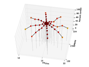
Figure 10 and Figure 11 show the results (with and without the pitch cutoff, respectively) for the features generated from the cycle-1 slice of the SSI. Overall performance with no pitch cutoff is 79.0%, and 81.3% with the pitch cutoff. In the no pitch cutoff case, performance is again lowest for the speaker with the shortest vocal tract, falling to 27.0%. For the pitch cutoff case, performance is lowest on the speaker with the longest vocal tract at 27.6%.

Figure 10 --- Scaled syllable recognition performance on the SSI cycle-1 profile with no pitch cutoff.

Figure 11 --- Scaled syllable recognition performance on the SSI cycle-1 profile with the pitch cutoff.

In general, then, when there is no background noise, performance with the SSI-based features is lower than for the NAP-based features, and the SSI-based features are more susceptible to changes both in pitch and in VTL. This is a somewhat surprising result, since to a large extent, the energy distribution in the SSI profile is the same as that in the NAP. Performance is still better than with the MFCCs without VTLN, however, where overall performance was 75.5%. Performance with the SSI features does not approach that of MFCCs with optimal VTLN at 99.2%.

Testing in noise

So far, the recognition experiments in this thesis have all been performed on clean audio data. However, how a system performs in noise is also an important consideration for practical speech recognition. As discussed above, the SSI is expected to provide a representation of the input signal which is more robust to interfering noise than a purely spectral representation like the smoothed NAP profile or the mel-frequency spectrum. This hypothesis was tested by training and testing the syllable recognition system in noise. The recogniser was trained on features generated from syllables presented in a background of noise at a range of levels, and then testing performance of the same recognition system on each noise level in turn, and recognition performance on the features was measured as a function of signal-to-noise ratio (SNR).

To create the noisy data set, the syllables in the database were mixed with pink (1 / f) noise using the `sox' sound processing tool. The normalised RMS level of the voiced portion of the syllable was used as the reference level to establish SNR. Stimuli were generated with SNRs from +42 dB down to 0 dB, in 6 dB increments. SSIs were generated from the input sounds using AIM-C, and MFCCs were generated using HTK, as before. The four different types of SSI features (whole SSI profiles and cycle-1 slices, with and without the pitch cutoff) were computed for all SNRs. MFCC features, with and without optimal VTLN, were also computed for all SNRs. HMMs were trained on the nine inner speakers from the spoke pattern, as before. However, in this case each training example was presented with an SNR picked randomly and uniformly from the complete range of SNRs. Testing was performed with all examples from the same SNR. As in chapter 2, a range of HMM configurations were tested. As before, the pattern of performance was found to be similar across a wide range of HMM configurations, and the results are presented on a representative point in the feature space where performance was found to be near optimal for all the feature types, in this case a 2-emitting-state HMM with 4 output components after 8 training iterations of the HMM.

Figure 12 shows overall recognition performance as a function of SNR for MFCC features, with and without optimal VTLN, and for the features from the AIM NAP. As in the case of clean speech, performance is low on the standard MFCCs due to their lack of scale-shift invariance, and is high for MFCCs with VTLN. For the features from the AIM NAP, performance is consistently slightly lower than for the features with VTLN, and the two curves follow the same trajectory as noise level increases.

Figure 12 --- Recognition results for the AIM NAP profile and MFCC features, where the model was trained and tested in noise.

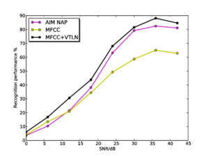
Figure 13 and Figure 14 show the results for the whole-SSI profile and SSI cycle-1 slice features respectively. In each plot, results are shown both with and without the pitch cutoff. In each case, the results vary very little depending on whether the pitch cutoff is used or not. In each case, there is a very slight benefit to using the pitch cutoff at high SNRs, but the cutoff is detrimental at low SNRs. This change is likely to be due to the simple algorithm used to compute the cutoff line, which just finds the highest peak in the temporal profile of the SAI, and takes this to be the most salient pitch in the input signal, making a hard decision on the input pitch. Once noise is added, this process will become less robust, and less consistent across different utterances so as the noise level increases the process starts to do more harm than good. A potential way of countering this effect would be to make a 'softer' pitch decision; this could take the form of a simple roll-off function that is applied to the edge of the SSI (for example a tanh window). The width of the roll-off could be modified depending on the pitch strength of the dominant signal pitch.

Figure 13 --- Recognition results for the whole-SSI profile AIM features, where the model was trained and tested in noise.

Figure 14 --- Recognition results for the SSI-slice profile AIM features, where the model was trained and tested in noise.

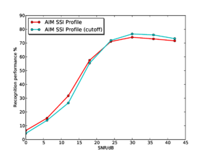
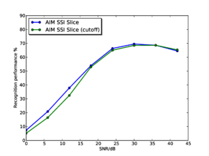
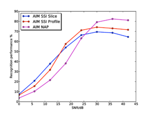
Figure 15 shows the results for the AIM SSI features (without pitch cutoff) and the AIM NAP features for comparison. Performance with the SSI-based features starts from a lower baseline, as as seen in the experiments on clean syllables. However, interestingly, performance degrades far less rapidly as the noise level increases for the SSI-based features, such that by 24dB SNR, the SSI-based features are outperforming the NAP-based features. Performance with the SSI-based features remains consistently higher right down the 0dB SNR. Furthermore, at SNRs of 12dB and below, the SSI slice-based features have the best performance, despite having started off with the lowest recognition rates in clean speech.

Figure 15 --- Recognition results for variants of the AIM features, where the model was trained and tested in noise.

Conclusions

The results with the SSI-based features suggest that there is indeed a benefit to using a representation of audio based upon the stabilised auditory image to improve noise-robustness in audio analysis tasks - however, baseline performance of the SSI-based systems is lower for clean input than that with simpler spectral-based representations. These results clearly point the direction for further research into the use of auditory models for content-based audio analysis tasks. The next step will be to explore whether it is possible to improve recognition performance on the SSI to bring it in line with that on the NAP alone. Initial inspection of the SSI profiles suggests that there is increased variability in these profiles relative to the smoothed NAP profile. This increased variability appears to be due in part to a feature of the strobed temporal integration process chosen to generate the images. In the version of strobed temporal integration used, SAIs are generated taking into account all strobe points which occurred before the snapshot of the auditory image is taken. This can lead to cases in which an SAI is generated when a strobe has recently occurred and only some data is available about what follows that strobe. If there is not enough signal available in a given channel to fill the complete width of the SSI, then the signal will be added up to the point where the signal stops, which can lead to small discontinuities in the generated image.

In the experiments in this chapter and in chapter 2, two important properties of auditory models have been demonstrated. First a macroscopic observed property of the auditory system, that it appears to perform automatic scale-normalisation, was used to inform the development of scale-shift invariance of the features. Secondly, a predicted property of the image stabilization process, that it creates auditory images which are more robust to interfering noise, was tested with the scale-shift invariant auditory features. However, these two properties of the auditory features are independent of one another, and it should be possible to demonstrate these two effects independently. One possible way to do this would be to summarise the spectral profile of the NAP and SSI by a more MFCC-like representation that does not have the scale-shift invariance properties of the Gaussian fitting procedure used in the above experiments. This could be done by taking a DCT over the logarithmically-compressed spectral profile of the NAP or SSI. Given the results presented above, the features generated from the SSI would be expected to be more noise-robust that those generated from the NAP.

Further work

In this chapter I have tested one possible feature representation generated from the SAI in a constrained task. However, there are many opportunities for creating a richer feature representation from the stabilised auditory image representation. Given the effectiveness of the DCT in lowering the dimensionality of the spectrum in MFCCs, a potential feature of interest might be created by taking the first DCT coefficient from each column of the SSI - generating a per-cycle MFCC-like representation. To include scale-shift invariance, the DCT could be replaced with a Fourier transform, and the phase discarded. Such features would correspond to a subset of the Mellin image (Irino and Patterson, 2002). These more general features could be assessed by trying them in a range of tasks where MFCCs are normally used.

Looking at the wider problem of how to process SAI-based representations into usable features, the major concern is how to perform dimensionality reduction in a manner which retains as much of the interesting information that it contains as possible while producing a feature vector which is sufficiently compact to be useful.

In chapter 6, one such system is developed: each SAI frame is decomposed into a set of blocks of different scales, and the contents of each block is converted into a sparse vector by use of a 'codebook' of common patterns seen in that block. This multi-scale approach to the problem of feature extraction is a crude but effective way of analysing different parts of the SAI in an independent manner, and removes the dependence of the current systems on the expensive fitting of spectral profiles with a constrained GMM. The feature representation developed in chapter 6 is considerably richer than these simple GMM-based features and allows for its use on a more open-ended task.