Auditory-Based Processing of Communication Sounds

From CNBH Acoustic Scale Wiki

Jump to: navigation, search

← Category:Auditory Processing of Communication Sounds

Thomas C. Walters

Introduction

The human auditory system is a remarkable signal processing device, which is optimised for the analysis of communication sounds in challenging acoustic environments. As I write this introduction, I am sitting in a crowded cafe; there are at least a dozen different conversations going on around me, music playing in the background, a noisy espresso machine in front of me, vehicles passing in the street outside and baby crying just to my right. From this cacophony I can trivially identify the various sound sources, and turning my attention to one of them and concentrating, I can follow a conversation, identify the song playing, or track the progress of an emergency vehicle down the street. This wealth of information comes from the analysis of a pair of waveforms by a combination of a dynamically-controlled 'hardware' system, in the form of the cochlea, and signal processing 'software' in the form of neurons all the way up the auditory pathway from the cochlear nucleus to primary auditory cortex and beyond. The systems in our heads which perform this processing are the result of hundreds of millions of years of evolutionary fine-tuning, and we have only begun to understand how they work. However, just because we don't fully understand every aspect of auditory processing doesn't mean that we shouldn't try to put what we do know to good use.

Ever since computing devices entered the popular consciousness, there has been a rather anthropomorphic expectation that such machines should be able to parse complex auditory and visual scenes with ease. Such an expectation is not unreasonable; `If we can do these tasks so easily,' runs the train of thought, `then it must be trivial for these complicated computing machines.' Of course, nothing could be further from the truth. There is some decidedly non-trivial computation going on in our skulls. However, by learning what makes our own abilities so special, and then applying some of the tricks that we learn to the automated analysis of audio we hope to improve the performance of machine systems which attempt to understand some features of sound.

This thesis covers a few aspects of the still-nascent field of 'machine hearing': the application of models of human audition to the analysis of complex audio signals by machines. These models, which are sometimes very simplistic, are used to generate feature streams which can be passed to automated systems to extract meaning from sounds. Making use of some of the features of the auditory system which are believed to assist in the processing of communication sounds. This combination of physiological simulation and engineering application is not new. For example, the quasi-logarithmic mel frequency scale employed by mel-frequency cepstral coefficient (MFCC) features (which are ubiquitous in content-based audio analysis) is based on observations about human pitch perception. However machine hearing is based far more upon the systematic application of knowledge and results from the study of human hearing to audio analysis problems.

In this thesis the auditory image model (AIM), is used as the basis of the auditory model. Two different feature representation are developed and tested. One on a simple speech recognition task, the second on a more complex sound-effects analysis task. As part of this undertaking, the physiological basis of auditory processing is reviewed, and used to inform improvements to various parts of AIM. As a test of the features produced, AIM is used as a preprocessor for an automatic speech recognition system and an audio search engine.

AIM is an existing computational model of human auditory processing. It simulates the processing which goes on in the early stages of the human auditory pathway, and its design is informed by the physiology of the auditory system. In this thesis, aspects of AIM are developed and refined for use in machine hearing, both by the use of data on human physiology and perception, and by the application of prior knowledge of the structure of communication sounds. The representations of sound generated by AIM are further processed to produce sets of features which describe perceptually-salient aspects of the input sound. Two machine hearing systems are developed; these systems use the auditory features produced by AIM in a speech recognition task and a sound-effects search task. Significantly, the systems are able to scale to large datasets, allowing the use of auditory features in machine learning tasks requiring hundreds of hours of training data.

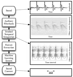
Figure 1 – Left: Structure of the auditory image model when used as a preprocessor for machine hearing applications. Right: Content / results of the various processing stages

Figure 1 is a block diagram showing the overall structure of the auditory image model when used as a preprocessor for machine hearing applications. This thesis concerns itself with all sections of the model, from the input audio to the machine learning system. This introduction provides an overview of the sounds used by animals to communicate, and outlines the structure of the systems which are described in more detail in later chapters; in particular, AIM is introduced in this chapter. Chapter 2 describes the use of a simple auditory filterbank to produce features for a syllable recognition task. The features generated are designed to be scale-shift invariant, mimicking an important feature of human perception of communication sounds. Chapter 3 deals with the generation of stabilised auditory images from the output of the cochlear model, and in particular the process of strobe detection for the strobed temporal integration process. Chapter 4 describes the generation of noise-robust auditory features by use of the stabilised auditory image (SAI) generated by AIM. The process of strobed temporal integration in AIM is found to create features which are more roust to interfering noise than simple spectral features. In chapter 5, various models of human auditory filtering are assessed; these models simulate the response of the outer and middle ear, the nonlinear response of the cochlea, and the neural transduction performed by the inner hair cells, leading to a simulation of the signal transmitted up the auditory nerve in response to any sound. Two different models of the compressive auditory filter are compared and improved by reference to the physiology of hearing and the constraints of the auditory model. Finally in chapter 6, a complete machine hearing system comprising a compressive filterbank, a stabilised auditory image, a sparse feature representation and a machine learning system is used as a sound-effects search tool which is capable of associating text terms with the content of audio files.

Communication sounds

Figure 2 – Cross-section of the human vocal tract, taken from Gray's Anatomy (Gray, 1918). The pulses are produced by the vocal folds, and these cause the vocal tract above to resonate.

The voiced parts of human speech take the form of pulse-resonance signals. The production mechanism for these sounds is simple: the vocal folds interrupt the stream of air from the lungs periodically, producing a stream of pulses which excite resonances of the vocal tract above the larynx. The form of the resonances carries information about the body which produced them. Figure 2 shows a cross-section of the human vocal tract; in human speech the configuration of the excited vocal tract, and thus the resonance pattern which it produces, carries information about the vowel which was spoken. This is the source-filter model of speech production (Dudley, 1939).

Pulse-resonance communication sounds are used as a primary means of communication, in one form or another, by most animals. The production system is similar in each case, a sharp pulse or series of pulses excites resonances in the body of the animal, and these resonances carry distinctive information about the shape and size of the resonating body (Patterson, Smith, van Dinther and Walters, 2008)<ref>For the first reference to publications that I have been personally involved with, I cite the author list in full to emphasise that I was involved in the work during the course of my PhD.</ref>.

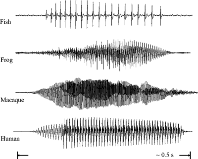
Figure 3 – Communication `syllables' of four different animals. They are the calls of a Jamaica weakfish (Cynoscion jamaicensis), a North American bullfrog (Rana catesbeiana), a macaque (Macaca mulatta) and a human adult saying the syllable /ma/. All the sounds in the figure may be heard on the CNBH acoustic scale wiki. The Jamaica weakfish call is originally from fishecology.org/soniferous/justsounds.htm. The bullfrog and macaque calls were kindly provided by Mark Bee and Asif Ghazanfar respectively.

Figure 3 (as published in Patterson et al., 2008) shows the communication 'syllables' of four different animals. Each 'syllable' is an example of a pulse-resonance sound. In each case the pulse-rate is different, and the form of the resonance following each pulse is different. The pulse rate determines the pitch of the sound, and the form of the resonance contains information about the shape and the size of the resonating structures in the body of the animal.

The pulse production mechanisms used by the fish, the frog and the mammals in this example are very different. Both of the mammals use the vocal folds in the larynx to periodically interrupt the flow of air from the lungs. The frog pushes air between its lungs and an air sac, causing a resonance in its tympanic membrane (Purgue, 1997), and fish employ mechanisms such as swift contraction of a ring of muscle around the swimbladder (Sprague, 2000).

In addition to human and animal vocalisations, van Dinther and Patterson (2006) suggest that the sounds produced by sustained-tone instruments can also be well modelled as pulse-resonance sounds. This means that a wide range of the sounds which are encountered by humans in their everyday life take this form.

Size information in communication sounds

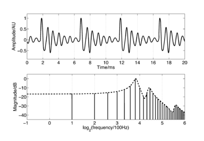
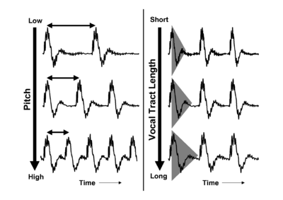
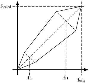
Figure 4 – Waveform and spectrum of a synthetic /a/ vowel as might be spoken by a child

When a pulse excites resonances in the body of a calling animal, the form of the resonances provides information about the resonating body. The shape and structure of the body make a major contribution to the form of the resonance, but so too does the overall size of the resonating body. If two animals of the same species make the same call, then the major factor that distinguishes the two calls will be the sizes of the calling individuals. Figure 4 shows a short section of the waveform (upper panel) and spectrum (lower panel) of a synthetic /a/ vowel, as might be spoken by a child. The waveform shows that the vowel is composed of a series of glottal pulses, followed by decaying resonances. The Fourier magnitude spectrum in the lower panel is shown as a set of vertical lines, and the spectral envelope is shown as a dashed line connecting the peaks of the magnitude spectrum. The shape of this envelope corresponds to the form of the damped resonance following each pulse, and the spacing of the harmonic peaks is determined by the pulse rate. As a child grows into an adult, the length of the vocal tract increases and the average glottal pulse rate (GPR) decreases as the vocal cords develop (Lee et al., 1999). Vocal tract length (VTL) increases in proportion to height (Fitch and Giedd, 1999; Turner and Patterson, 2003; Turner et al., 2009), and people approximately double in height from the time that they start speaking to the time they are fully grown, meaning that formant frequencies approximately halve over this time. An increase in vocal tract length causes the resonance following each pulse to ring longer and decay more slowly. In the frequency domain, this corresponds to a shift of the spectral envelope on a log-frequency scale. A decrease in glottal pulse rate causes the time between pulses to increase; in the frequency domain this leads to the harmonic peaks becoming more closely spaced. Figure 5 shows the waveforms for real human vowels, which have been scaled to simulate these changes in GPR (left) and VTL (right).

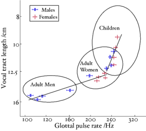
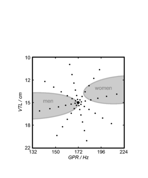
Figure 5 – Waveforms from a vowel showing the effects of changes in VTL and GPR.

A reanalysis of the classic formant data of Peterson and Barney (1952) by Turner, Walters, Monaghan and Patterson (2009) showed that the relative formant pattern that defines a particular vowel remains approximately unchanged as children grow into adults. Turner et al. also developed a technique to infer VTL values from the formant frequency data of Peterson and Barney and Huber et al. (1999) allowing them to plot the position of men, women and children in the GPR-VTL plane, and show the trajectories that humans pass through in the space as they develop. Figure 6 is taken from Turner et al.. The ellipses show the position of, from left to right, men, women and children in the GPR-VTL plane. They are plotted at two standard deviations, so they enclose around 80% of the speakers in that particular class. The solid lines are regression lines though the data points from Huber et al.. All speakers, boys and girls, start off at the top right of the space, as boys and girls grow up, their voices develop in the same way initially, but at puberty there is a sudden drop in pitch in the boys' voices and they end up moving very quickly to their final position with a much lower GPR and slightly longer VTL than women.

Size information is also seen in the calls of animals, for example there is a strong correlation between the body size of the North American bullfrog (Rana catesbiana) and the fundamental frequency of its call (Gomersall, Walters and Patterson, 2005).

Figure 6 – The VTL-GPR plane. Ellipses show the position of adult men, adult women and children in the space. The lines show the developmental path as children grow into adults, and the individual red and blue data points show the VTL-GPR combinations for males and females at different ages. This figure is adapted from figure 13 in Turner et al. (2009)

The scaling of communication sounds

STRAIGHT (Kawahara and Irino, 2004; Kawahara et al., 1999) is a high-quality vocoder that is capable of analysing speech with glottal-cycle resolution. STRAIGHT's processing scheme is based on the classic source-filter model of speech production (Dudley, 1939). Speech sounds are modelled as being a stream of glottal pulses, the source, which pass through the vocal tract, the filter. STRAIGHT is able to independently extract the pitch track and the spectral envelope from human vocalisations. The pitch track and spectral envelope can then be manipulated independently before the sound is re-synthesised. Using STRAIGHT it is therefore possible to scale human vocalisations in the GPR and VTL dimensions independently. This has proved an invaluable tool for research into both human perception and normalisation of communication sounds (Ives, Smith and Patterson, 2005; Smith and Patterson, 2005; Smith, Patterson, Turner, Kawahara and Irino, 2005; Smith, Walters and Patterson, 2007; Walters, Gomersall, Turner and Patterson, 2008) and into speaker-independent automatic speech recognition (Monaghan, Feldbauer, Walters and Patterson, 2008; Feldbauer, Monaghan and Patterson, 2008).

STRAIGHT works by first extracting a pitch, or fundamental frequency ( $f 0$ ) track for a sound. This is done by a combination of spectral and temporal analysis. In the frequency domain, instantaneous $f 0$ extraction is performed using an analysis wavelet that encodes prior information about the expected shape of the distribution of harmonics in a voiced speech sound. This is combined with a time-domain normalised autocorrelation analysis to reduce $f 0$ errors. Once an accurate pitch track has been extracted, the sound is re-analysed using a pitch-synchronous window. Typically when a periodic sound is analysed using a short-window Fourier transform, the periodicity of the waveform and the window size interfere to create a periodic temporal structure in the extracted spectrogram. STRAIGHT uses a smooth windowing function that is temporally modulated with the periodicity of the incoming audio signal. This leads to a temporally smooth spectrogram. The harmonic structure of the spectrogram is then removed using a spline-based smoothing technique, leaving the reconstructed spectral envelope, independent of the pitch.

Human perception of size

Humans are remarkably good at understanding the content of vocalisations that come from a wide range of speakers. Smith, Patterson, Turner, Kawahara and Irino (2005) demonstrated that humans could accurately identify vowel sounds that had been scaled to VTL and GPR values well outside the range of normal experience. In that study, Smith et al. presented scaled versions of five human vowels (/a/, /e/, /i/, /o/ and /u/) to human subjects in a 5-alternative forced-choice experiment. The vowels were scaled in GPR and VTL using the vocoder STRAIGHT (Kawahara et al., 1999). The scaling encompassed VTL values corresponding to humans from one-third the height to twice the height of an average man, and GPR values from 10Hz to 640Hz. At 10Hz, the sounds were below the lower limit of pitch, but subjects were still able to detect the vowel type from the individual pulses and resonances. Smith et al. found that combined recognition performance fell to 50% (still better than chance) only at the very far extremes of the GPR and VTL range, despite the fact that these are well outside the range of normal experience. While it is possible that humans simply learn to recognise speech by hearing examples from a wide variety of sizes of speaker, the fact that recognition performance continues to be high well outside the range of normal experience suggests that there may be some sort of automatic size-normalisation system within the human auditory system.

Ives et al. (2005) extended the stimuli from the study of Smith et al. (2005) to a large database of 180 consonant-vowel and vowel-consonant syllables. They again showed that recognition performance was extremely good across the entire range of GPR and VTL; indeed, performance was better than for the vowels alone.

In a related study, Smith and Patterson (2005), again using scaled vowels, demonstrated that VTL has a strong effect on the perception of speaker size. In this experiment, listeners were asked to judge the height of a speaker with a given combination of GPR and VTL on a seven-point scale from 'very tall' to 'very short'. Listeners were also asked to judge the sex and the age of the presented speakers from four choices: 'man', 'woman', 'boy' and 'girl'. Size judgements were strongly affected by VTL and only slightly affected by GPR. Sex and age judgements for vowels with GPR and VTL values in the range of normally-encountered speakers were influenced about equally by both variables, but for vowels with low GPR and short VTL, VTL played a greater role in the decision.

Extending from this study, Walters, Gomersall, Turner and Patterson (2008) attempted to identify the 'trading relationship' between VTL and GPR in making judgements of speaker size. Listeners compared sequences of vowels scaled in GPR and VTL to represent speakers with slightly different sizes. The experiment was of a two-alternative forced-choice design, in which subjects were required to choose the interval with the smaller speaker. By comparing speakers around a point in the GPR-VTL plane, an estimate of the gradient of the VTL-GPR plane at that point was made. The vectors across the GPR-VTL plane were integrated to estimate the size surface. The results indicated that the size surface would be essentially planar if determined by size discrimination alone. This suggests that relative size judgements are different from absolute size judgements.

The stimuli in all the above experiments were synthesised from a single speaker. Smith, Walters and Patterson (2007) investigated the role of the input speaker on the perception of speaker size. In this study, sustained vowels from men, women and male and female children were scaled using STRAIGHT to a range of VTLs and GPRs. Subjects were then asked to identify whether they thought the vowel had come from a man, a woman, a boy, or a girl. Smith et al. found that while the sex of the input speaker did not make a significant difference to the judgement, the age of the speaker did. This prompted them to suggest that the differences in the ratio of the sizes of the oral cavity and pharynx between children and adults may account for the difference. However, vowel formant ratios are known to remain largely fixed as children grow up. Taken together, these two pieces of evidence suggest that speakers may actively vary the position of their tongue in the oral cavity to maintain a fixed formant ratio, regardless of anatomical differences.

van Dinther and Patterson (2006) performed a similar study to those described above, but used musical instrument sounds as the input pulse-resonance signals for size discrimination. They demonstrated that, as with human vocalisations, subjects were able to detect relatively small changes in the scale of the resonance in the notes of sustained tones from string, woodwind and brass instruments, and singing voices. This suggests that the normalisation mechanisms at work may be the same for human voices and for other pulse-resonance sounds.

The problem of automatic vocal tract length normalisation (VTLN) is an area of active research in speech recognition. Approaches to VTLN include warping the frequency spectrum of the input sound before feature computation (Welling et al., 2002) to more complex systems such as cross-correlation of the spectra at various points in time to extract a locally-normalised spectrum (Mertins and Rademacher, 2005). Inspired by the observation that humans appear to be able to perform VTLN automatically on the incoming signal, in chapter 2, an alternative feature representation for machine hearing which is invariant to changes in the size of the source is developed and tested.

The auditory image model

The auditory image model (AIM) (Patterson et al., 1992; Patterson et al., 1995) is a computational model of auditory processing. It is the basis for most of the work in this thesis. AIM is a functional model of the signal processing performed in the auditory pathway; it consists of modules which simulate the stages of processing which occur as the system converts a sound wave into the initial percept which a human experiences when presented with a sound, but before any semantic meaning is attached to the sound. The first three stages of the model simulate the effect on the signal of the outer and middle ear, the cochlea, and the hair cells which translate the motion of the cochlear partition into neural impulses. These stages are all based on the physical properties of the various structures and systems which perform the processing. The subsequent stages of the model are based less upon observations of the physical processes and more upon observations of human perception of sounds. These latter stages convert the incoming sound into a 'stabilised auditory image' (SAI). This is a representation in which sounds that are perceived as stable by humans give rise to stable auditory images. The SAI is a 'movie' with 2-dimensional frames along the time dimension; each frame has two dimensions: cochlear channel and time interval. The pulse rate (pitch), the resonance scale (size) and the form of the resonance (the message) of the incoming sound are segregated as far as possible into covariant dimensions in this representation.

The human auditory system

The human auditory system is an immensely powerful signal processing system. It can deal with sounds from a whisper to a rock concert -- over 10 orders of magnitude difference in intensity (Moore, 2003) -- and it can extract meaning from sounds which have been heavily degraded by the addition of background noise or sounds from competing sources (Miller and Licklider, 1950). The anatomy of the peripheral auditory system is illustrated in Figure 7.

One of the central premises of this thesis is that a great deal may be learned from the auditory system about the best strategies for the extraction of salient information from sounds. Models of aspects of auditory processing are used as the basis for audio compression schemes including MP3 and AAC (Brandenburg and Stoll, 1994; !! Unknown ref iso:1993 !!; !! Unknown ref iso:1997 !!) and auditory models have been recommended for the enhancement and segregation of speech sounds in noisy environments (Slaney et al., 1994; Irino et al., 2006). However, the standard features used for content-based audio analysis tasks, such as speech recognition (Young et al., 2005) and music information retrieval (Bergstra et al., 2006), are usually based on the more simple short-window Fourier transform as a first processing step.

Figure 7 – Anatomy of the human ear. Originally by Chittka L. Brockmann. Used under Creative Commons Attribution 2.5 Licence

Example stimuli

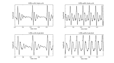
Figure 8 – Short sections of the waveform for four examples of the vowel /a/. In the upper panels are vowels as might be spoken by a person with a vocal tract length (VTL) of around 12.7cm; in the lower panels, the VTL is around 17.5cm. In the left panels, the glottal pulse rate (GPR) is 110Hz and in the right panels the GPR is 256Hz.

In the next few sections, the workings of AIM will be discussed. In order to illustrate each stage, four STRAIGHT-scaled vowel sounds will be processed using the model, and plotted side-by-side for comparison. The four vowels are shown in Figure 8; each is an /a/ vowel. Each subfigure of Figure 8 shows the waveform from a different speaker uttering the vowel sound. In the lower subfigures, the waveforms have a resonance rate of 89% of that of the original speaker. This corresponds to a person with a VTL of approximately 17.5cm or of height of 194cm. In the upper subfigures are the waveforms for a resonance rate of 122% (VTL 12.7cm; height 142cm). The left subfigures are for a GPR of 110 Hz and the right subfigures for a GPR of 256 Hz.

Outer and middle ear

The first structures of the auditory system which are encountered by an incoming sound wave are the outer and middle ear. The pre-cochlear processing (PCP) module applies a filter to the input signal to simulate the transfer function from the sound field to the oval window of the cochlea. The purpose is to compensate for the frequency-dependent transmission characteristics of the outer ear (pinna and ear canal), the tympanic membrane, and the middle ear (ossicular bones). At absolute threshold, the transducers in the cochlea are assumed to be equally sensitive to audible sounds, so the pre-processing filters apply a transfer function similar to the shape of hearing threshold. The default version of PCP applies the function described by Glasberg and Moore (2002).

The cochlea

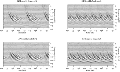
Figure 9 – Basilar membrane motion plots for the four vowels shown in Figure 8. The horizontal axis in each panel is time, as before. The vertical axis is cochlear channel, from low frequency at the bottom to high frequency at the top. A 50-channel dynamic compressive gammachirp (dcGC) filterbank, with filter centre frequencies ranging from 100Hz to 6kHz on an ERB scale was used to generate the figures.

The basilar membrane motion (BMM) module in AIM simulates the spectral analysis performed in the cochlea with an auditory filterbank. Figure 9 shows the output of the AIM BMM module for the four input sounds from above. The output of the BMM stage is a multi-channel representation of the incoming sound; the output channels correspond to the motion over time of points spaced equally along the length of the basilar membrane. The configuration of the basilar membrane is such that equally spaced points respond preferentially to frequencies which are spaced along a quasi-logarithmic scale such as the ERB scale (Smith and Abel, 1999). There is essentially no temporal averaging, in contrast to spectrographic representations where segments of sound 10 to 40 ms in duration are summarised in a spectral vector of magnitude values. There exist several different filterbanks in AIM; the default, the gammatone (Patterson and Moore, 1986), is a passive linear filter which does not simulate any of the level-dependent properties of auditory filtering. More realistic and more complex models of the auditory filter are provided by the dynamic compressive gammachirp (dcGC) (Irino and Patterson, 2006) and pole-zero filter cascade (PZFC) (Lyon et al., 2010). Both of these models include level-dependent asymmetry, and fast acting compression. The BMM plots in Figure 9 were generated using the dcGC filterbank. In the plots, time runs along the horizontal axis, and cochlear channel is along the vertical axis. The higher-frequency cochlear channels are at the top of the plot. The pulse-resonance structure of the vowel sounds is clearly visible; the pulses excite filters at all frequencies, leading to a periodic curved ridge in the plots. For the high glottal pulse rate (right panels), the pulses occur more frequently. After the pulse, the filters in all channels then ring. The resonances that follow the pulses in the input sound put energy into the filters at some frequencies, causing them to ring for longer and decay more slowly. These resonances are the formants of speech. For the short VTL (upper panels), the entire pattern of formants is shifted up in frequency and decays faster in time. Chapter 5 investigates the benefits of using a compressive filterbank for the task of pitch detection.

Neural activity pattern

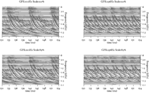
Figure 10 – Neural activity patterns generated from the basilar membrane motions shown in Figure 9 for the four example vowels. Here, the output of the dcGC filterbank is half-wave rectified and low-pass filtered (but no further compression is applied).

The basilar membrane motion is converted into a simulation of the neural activity pattern (NAP) observed in the auditory nerve using a model of the neural transduction that occurs in the hair cells of the cochlea. The most important feature of this stage is that the signal is half-wave rectified, mimicking the unipolar response of the hair cell, while keeping it phase-locked to the peaks in the wave. Experiments on pitch perception indicate that the fine structure retained by phase-locking is required to predict the pitch shift of the residue (Yost et al., 1998). Other rectification algorithms like squaring, full-wave rectification and the Hilbert transform only preserve the envelope. At this stage, it is also possible to apply compression to the waveform. The compression is intended to simulate the cochlear compression which is essential to cope with the large dynamic range of natural sounds.This compression is already present in the dcGC and PZFC filters, but is absent in the gammatone filters. Figure 10 shows the results of NAP processing on the four vowels.

Strobed temporal integration

Figure 11 – A dynamic threshold applied to each NAP channel individually is used to identify strobe points.

The next stage of the model is the identification of significant or `strobe' points in the NAP. Perceptual research on pitch and timbre indicates that at least some of the fine-grain time-interval information in the NAP survives to later stages of the auditory pathway (Krumbholz et al., 2003; Patterson, 1994a; Patterson, 1994b; Yost et al., 1998). This means that the temporal integration that occurs in the auditory system cannot be simulated by a running temporal average process, since averaging over time destroys the temporal fine structure within the averaging window (Patterson et al., 1995). Patterson et al. (1992) argued that it is the fine-structure of periodic sounds that is preserved rather than the fine-structure of noises, and they showed that this information could be preserved by finding peaks in the neural activity as it flows from the cochlea, measuring time intervals from these strobe points to smaller peaks, and forming a histogram of the time-intervals, one for each channel of the filterbank. This two-stage temporal integration process is referred to as strobed temporal integration (STI). The strobe-point-finding (or 'strobing') process identifies certain peaks in the NAP and the timings of these strobe points are used to initiate a temporal integration process in the following stage. The strobe pulses enable the segregation of the pulse and resonance information and they control pulse-rate normalisation. For ideal pulse-rate normalisation, the chosen NAP peaks should correspond to the onset of a pulse in the input sound. However, auditory image construction is robust, in the sense that strobing does not have to occur exactly once per cycle to be effective.

Strobe detection in AIM is performed using a dynamic thresholding technique. Figure 11 shows the 'parabola' dynamic thresholding algorithm applied to a NAP. A threshold which decays linearly over time is placed on the signal; when the signal exceeds the threshold a strobe point is issued, and the threshold rises briefly above the level of the signal at that point. The threshold then decays again until it meets the signal and the process repeats. This has the effect of causing strobes to be issued only on certain peaks in the NAP.

Figure 12 – Strobe points overlaid on the four NAPs in Figure 10

Figure 12 shows the results of applying the same algorithm to the NAP output for the four vowels. The strobe points clearly cluster around the glottal pulses, but they do not occur exclusively at those times.

The SAI module uses the strobe points to convert the NAP into an auditory image, in which the pulse-resonance pattern of a periodic sound is stabilised using the strobe points generated in the previous stage.

The 'ti2003' algorithm is the default method for generating SAIs in the software packages AIM-MAT and AIM-C (which are discussed below). It works in the following way. When a strobe occurs it initiates a temporal integration process during which NAP values are added into the corresponding channel of the SAI as they are generated; the time interval between the strobe and a given NAP value determines the position where the NAP value is entered in the SAI. In the absence of any succeeding strobes, the process continues for 35ms and then terminates. If more strobes appear within 35 ms, as they usually do in music and speech, then each strobe initiates a new temporal integration process. Each process is given a weight with which NAP values from that process are added to the SAI. Initially these weights are inversely proportional to the index of the strobe in the series so, for example, if there are three active strobes, the oldest strobe is added with weight 1/3 relative to the most recent strobe which is added with weight 1. Finally, the weight set is normalised to sum to unity so that the overall level of the auditory image is normalised to that of the NAP.

STI converts the time dimension of the NAP into a time-interval dimension in the stabilised auditory image (SAI). A series of vertical ridges appear in the auditory image. These are associated with the repetition rate of the source and can be used to identify the start point for any resonance in that channel. It is this property which makes it possible to segregate the glottal pulse rate from the resonance structure of the vocal tract in the SAI.

In chapter 3, the properties of an 'ideal' strobe detection system are defined, and a number of strobe detection systems are presented and analysed based on this definition.

Figure 13 shows the results of the STI process for the four vowels. The zero-lag point is not shown in this representation, but the vertical ridge due to the pulse rate of the original waveform is clearly visible, and can be seen to shift as the pulse rate changes. The formants appear as 'flags' running horizontally from the vertical pitch ridge. The formats shift up in frequency and get narrower in the time-interval dimension from the long VTL waveforms to the short VTL.

Figure 13 – Stabilised auditory images (SAIs) generated from the four sounds in Figure 8. The horizontal axis is now time interval rather than time.

The STI process can be thought of as a modified form of autocorrelation. In autocorrelation, a signal is cross-correlated with itself to yield a measure of how well-correlated the signal is with itself when delayed by a range of different `lags'. Zero-lag is at the centre of the output, and the function is symmetrical about this point. In STI, the signal is instead cross-correlated with a function that is zero everywhere except at the strobe points. The height of the signal at these strobe points determines the weight with which that time interval is represented in the output. The process is less computationally intensive than autocorrelation, as one of the signals is sparse, being composed mostly of zeros. Unlike autocorrelation, the resulting output is no longer symmetrical about the zero-lag point (Irino and Patterson, 1997), and any temporal asymmetry in the input signal is preserved. This is an important feature of the SAI, as temporal asymmetry is a key feature of pulse-resonance sounds (Patterson and Irino, 1998). Figure 14 shows correlograms for the four vowel sounds. The zero-lag line is at the left of the image. Each of the structures due to the pulse repetition rate is more symmetrical in the correlogram than in the stabilised auditory image.

Figure 14 --- Correlograms (positive side only) for the four vowel sounds. Note that the correlogram representation is more symmetrical than the stabilised auditory image. The correlograms were generated by processing the AIM NAP output using Slaney's auditory toolbox (Slaney, 1993e).

It is worth noting that a huge increase in the data rate passing through the model takes place as the waveform is converted to a SAI through the AIM processes. In a standard simulation, a single time-domain waveform might be split into 50 time-domain channels, each with the same data-rate as the original waveform. SAIs can then be generated from these data at an arbitrarily high rate. Superficially, this seems like an extremely wasteful set of transformations to perform on a signal, but the benefit of this approach is that the space that the signal lies in after these transformations has the property that the pulse-rate and resonance information appear into two largely orthogonal dimensions -- a key property of the auditory model. The challenge in using such a representation for content-based audio analysis tasks is to reduce this data rate to a manageable level in a principled way, so that the useful properties of the space are preserved, but the feature size is not overwhelming for whatever machine learning system is subsequently used. Chapters 4 and 6 of this thesis examine two approaches to performing this data rate reduction.

Software

The two major software tools used in this thesis are AIM-MAT (Bleeck et al., 2004) and AIM-C, the MATLAB and C++ implementations of AIM. The implementations are in many ways complementary. AIM-MAT provides an environment in which processing modules can easily be tested and compared, and it makes it extremely easy to visualise the results of processing. AIM-C by contrast provides capabilities for the fast processing of long audio files through a pre-prepared set of modules. Both AIM-MAT and AIM-C were written in the CNBH lab in Cambridge. AIM-MAT was written by Stefan Bleeck and was released in 2004. I wrote AIM-C between 2006 and 2009. I worked on the initial design and much of the early infrastructure code with Willem van Engen, a Masters student whom I supervised in 2006.

Both AIM-MAT and AIM-C have a modular architecture. The individual stages of the auditory image model (PCP, BMM, NAP, Strobes and SAI) are implemented as separate, interchangeable modules. With this design, it is simple to write and test individual modules for the different stages of processing, and to easily test different combinations of these modules. In AIM-MAT it is possible to easily visualise the output of the different modules by use of the graphical user interface. The main motivation for the development of AIM-C was to improve the speed of processing available. One major design limitation of AIM-MAT is that all the processing for one module is performed before the next module, so if a long sound is processed it must be run in its entirety through the BMM module, for example, before being passed on to the later modules. This means that the entire processed output must be stored in memory at each stage. Given the massive increase in data rate that happens at the BMM and SAI stages of the model, this means that only short sounds (on the order of a few seconds) can be processed before the host computer runs out of RAM. AIM-C, by contrast, has a block-based 'pipeline' architecture in which short segments of the audio are processed through each stage of the model in turn, and stored only at the end. This allows AIM-C to process arbitrarily long pieces of audio, limited only by the available hard drive space of the host machine. AIM-C is also significantly faster at processing sounds, since it is written in C++ rather than MATLAB. On a modern machine, AIM-C is capable of processing audio in realtime, with a 30-channel filterbank, and displaying the generated SAI with only a short delay of around 50ms.

AIM-C includes modules for the gammatone, dcGC and PZFC filterbanks and for various strobed temporal integration algorithms. The filterbank implementations in AIM-C run considerably faster than the equivalent versions in AIM-MAT. In general, there is at least an order of magnitude improvement in speed available in using AIM-C over AIM-MAT. This speed increase is crucial when processing large datasets. It is AIM-C that made it possible to perform the syllable recognition studies presented in chapters 2 and 4.

Invariance properties of the auditory system

The auditory system has two important invariance properties in its processing of sounds. The first is that it is time shift invariant: the sound we hear is independent of the time that it occurs<ref>From a perceptual point of view, it is not necessarily always the case that the auditory system is fully time-shift invariant; the experiments of Ladefoged and Broadbent (1957), for example, demonstrate that perceptual effects can come into play depending on the relative timing of stimuli. However, these effects occur at a much later stage in the auditory pathway.</ref>. The second property is that, over a wide range of values, it is scale invariant with respect to the message: the same message can be perceived over a range of time-scalings of the input signal.

Time-shift invariance may seem obvious, but it is an important property of the system and leads to certain mathematical constraints. In the case of a time-scaling of the signal, there is a clearly perceptible change in the sound itself, but the message information itself is relatively unaffected by the scaling.

In its simplest form, scale invariance can be seen as an invariance to changing the 'tape speed' of a signal. Imagine a tape or vinyl recording of speech which is played back at the wrong speed. For a wide range of playback speeds, it is still easily possible to discern what the speaker is saying, even if other characteristics of the voice (such as the perceived size or age of the speaker) may change wildly. This is an important observation, as it encompasses both aspects of the size normalisation which we believe that the auditory system must perform. The 'tape speed transform' simultaneously simulates a change in glottal pulse rate, a corresponding change in vocal tract length and a change in the rate of speaking. However, it is also possible for these three properties to change independently: a speaker changes the pitch of their voice through an utterance, people with different vocal tract lengths may speak the same phrase with the same pitch, and the same sentence may be uttered at a faster or slower rate. For the purposes of investigating the properties of the early stages of the auditory system, it is only the first two of these properties that are of interest to us since longer-term temporal variations are dealt with at a later stage of processing. Given the observation that the pulse rate and the resonance scale of the system can vary independently, but lead to the same message being perceived, the invariance properties of the system must be more complex than simple time-scale invariance, as the system is invariant to changes in scale on the longer time scale of glottal pulse rate and to changes in the microstructure of the resonances that the glottal pulses excite.

One conclusion from these observations could be that the system must perform some form of deconvolution of the glottal pulses from their associated resonances. In the auditory image model, this deconvolution occurs at the strobe-finding stage. Furthermore, there must be some process that is able to normalise the signal both for changes in pulse rate and changes in resonance scale. In the SAI changes of pulse rate correspond to a change in the horizontal spacing of the vertical pitch ridges, and changes of resonance scale correspond to changes in the vertical position of the resonance structure. So, to a certain extent, the SAI segregates the two forms of scale information into two dimensions of the auditory image. The SAI is also a reasonable representation from a physiological point of view. A two-dimensional frequency-periodicity mapping, like that seen in the auditory image and the correlogram, has been observed in the inferior colliculus of the mammalian brain (Schreiner and Langner, 1988).

The 'size-shape' image (SSI), introduced in chapter 4, processes the SAI further by truncating the signal in each channel after the first pitch ridge, and by scaling the time axis of each channel independently by an amount proportional to the centre frequency of the filter in that channel. This produces a representation that is, as far as possible, pitch invariant and is scale-shift covariant; changes in resonance scale correspond to a simple shift of the image in the vertical dimension. The question of how best to transform the SSI from a pitch-invariant, scale-shift covariant representation to a pitch-invariant, scale-shift invariant representation is still an open one. The Mellin image (Irino and Patterson, 2002) has been suggested as a possible scale-shift invariant representation. The techniques employed in chapters 2 and 4 (to generate features from auditory models for a speech recognition system) produce a representation of the spectral profile of the auditory image that is scale-shift invariant.

Time-frequency and time-scale uncertainty relations

The short-time Fourier transform (STFT) is a joint time-frequency representation of a signal: it transforms a 1-dimensional signal into a 2-dimensional time-frequency representation. Using methods from operator theory, it is possible to show that there is an uncertainty relation between time and frequency (since the time and frequency operators have a nonzero commutator), and it is possible to derive the set of functions which satisfy the conditions for minimal uncertainty. In the case of the joint time-frequency representation, the minimum uncertainty function is the Gabor function. Similarly, Cohen (1993) has investigated operator methods for a joint time-scale representation of a signal, where scale is seen as a physical property of the signal, just like frequency. Irino and Patterson (Irino and Patterson, 1997) employed these methods in their development of the gammachirp auditory filter. The gammachirp is in fact the minimal uncertainty function for a joint time-scale representation of a signal.

MFCCs

When designing new representations of sounds for content-based analysis, it is important to understand the systems which are currently used for these tasks. Mel-frequency cepstral coefficients (MFCCs) (Mermelstein, 1976; Davis and Mermelstein, 1990; Bridle and Brown, 1974) have been used for years as one of the primary representations of audio for speech recognition (Huang et al., 2001) and speaker recognition (Ganchev et al., 2005), and have found applications in many other content-based audio analysis tasks such as music genre classification (Bergstra et al., 2006). MFCCs have some excellent properties: they are cheap to compute, they produce coefficients that are reasonably independent of one another (a useful property for many machine-learning systems), and they have been applied extremely successfully to many applications.

MFCCs are calculated by taking the Fourier spectrum of a short, windowed portion of a signal (typically around 25ms). The frequency spectrum is then mapped onto the mel scale (Stevens et al., 1937) by means of a bank of triangular filters, and the logarithm of the power at each of the mel frequencies is taken. A discrete cosine transform (DCT) is then performed on the log filterbank output. This transformed representation is known as the `cepstrum' (a play on the word `spectrum'). Taking the logarithm of the power spectrum means that a convolution in the time domain corresponds to summation in this log-frequency domain. This is a useful property, since if the input audio is a pulse-resonance sound, in which a train of pulses is convolved with a resonance, then the log-spectrum can be viewed as a sum of the contribution from the pulse train and a contribution from the filter. This summation property also holds for the cepstrum. Akin to filtering in the frequency domain, `liftering' can be applied in the cepstral domain. Typically the mel-frequency cepstrum is low-pass liftered by discarding all but the lowest DCT coefficients (in many standard implementations, the first 13 coefficients are retained). These DCT coefficients are the mel-frequency cepstral coefficients. The low-pass liftering of the cepstrum removes much of the harmonic structure present in the original spectrum, meaning that the MFCCs capture the overall spectral shape of a sound well, but they are not very sensitive to pitch.

This thesis

In this thesis, I evaluate and develop some of the many aspects of the auditory image model, with a focus on using AIM to generate features that provide useful and salient information about the content of sound to machine learning systems. To do this, it is necessary to find a balance between accurately simulating the physiology and developing practical systems. In order to make these decisions, it is necessary to have a good understanding of the properties of all aspects of the system that might help them improve audio analysis tasks. In this thesis, I model a number of properties of the auditory system, from macroscopic, behavioural observations, right down to the analysis of fine timing in the cochlea, and assess systems based on these models on audio analysis tasks. As the observations and investigations become more low-level, the mode of evaluation changes, but the goal is to gain useful information about the behaviour of the system at each level. Finally, a complete audio analysis system is constructed which draws together many of the aspects investigated in the previous chapters. In this thesis I do not, and could not, attempt to assess the effect of every minute parameter change in every subsystem on the overall behaviour of a larger machine hearing system, but rather to assess some of the individual subsystems at the level at which it is most useful to do so.

In chapter 2, a simple syllable recognition system is developed which has the important property of scale-shift invariance. The scale-shift invariant features were motivated by the observation that human listeners can apparently automatically normalise communication sounds for differences in source size. The system uses a linear gammatone filterbank, which is a good first approximation to the cochlear filterbank, but which lacks the fast-acting compression which is known to exist in the cochlea. This system also makes no attempt to use the strobed temporal integration from AIM. This system is an initial proof-of-concept which demonstrates the potential utility of modelling a high-level aspect of auditory processing.

In chapter 3, the strobed temporal integration process is reviewed, refined and then in chapter 4, it is put to use to improve the noise-robustness of the experimental system described in chapter 2, demonstrating one of the benefits of the stabilised auditory image representation.

Chapter 5 deals with producing a system that accurately models the compressive properties of the human cochlea. Based on the observation that compressive filterbanks are able to more accurately model the human perception of stimuli with a weak pitch cue, the effectiveness of a pitch-strength detection system is tested using the linear gammatone filterbank, and the compressive dcGC and PZFC filterbanks as the cochlear front-ends for the model.

In chapter 6, a complete sound analysis system is constructed and analysed. The system uses AIM in one of its variants to generate features from audio to pass to a machine learning system. The technology has not previously existed to run AIM-like models on large databases of sounds. In AIM-C and the machine hearing systems developed at Google, we now have the technology to investigate the application of AIM to large-scale problems. This is an important and notable step forward in the field. Previously the use of AIM had been limited to the analysis of small datasets. The system described is able to process days of audio data in a matter of a few hours by the combination of efficient code and large computing resources.

The overall goal is to define and build a system that can be used for real applications. The system must model the processing performed in the auditory system with a degree of fidelity that reflects the aspects of auditory processing which make it robust and effective in processing communication sounds. However, it must still be possible to implement the system for use in practical applications which benefit from the improved auditory processing.

Footnotes

Scale-shift Invariant Auditory Features

The introductory chapter showed how pulse-resonance communication sounds could be normalized for acoustic scale, both in terms of the pulse-rate and the resonance-scale, and papers from the perceptual literature were presented which suggested that the human auditory system includes some form of automatic scale normalisation for both pulse-rate and resonance-scale. This chapter describes a method for extracting scale-shift invariant features using an auditory model and a simple syllable-recognition system designed to compare the value of these normalized auditory features with those commonly used in automatic speech recognition.

In this initial auditory model, the normalized feature representation is generated from the output of a simple, linear auditory filterbank without image stabilization. A linear filterbank provides a reasonable simulation of cochlear processing for wideband sounds that do not vary markedly in level which is the case for the syllable recognition task used to evaluate the normalized auditory features. The output of the simple cochlear model is passed to the feature-generation system with no attempt to model any further stages of the auditory processing, other than the higher-level property of normalization. This initial model is clearly overly simplistic, but it serves to demonstrate the value of automatic normalization for the processing of communication sounds, and it provides a baseline level of performance to compare with that achieved by a more complex machine hearing system described in a later chapter.

Introduction

In standard speech recognition systems, the acoustic features used to represent the speech change with the vocal tract length of the speaker. This means that a recognition system trained exclusively on utterances from one speaker with a fixed vocal tract length (VTL), or a fixed set of speakers with a limited range of VTLs, cannot be expected to generalise to the speech of speakers with arbitrary VTLs. By contrast, the human auditory system is exceptionally robust to changes in VTL, even when the test VTL is well outside the range of normal experience (Ives et al., 2005; Smith et al., 2005). In an attempt to improve the robustness of ASR, modern recognition systems often use a process of vocal tract length normalisation (VTLN) to warp the frequency spectrum of the incoming speech to bring the features more into line with those used to train the system (Welling et al., 2002). However, this process requires that the system optimise over a set of possible warpings of the frequency axis. A standard approach in such systems is to make two passes over the input waveform. In the first pass, the un-normalised version of the signal is used, and then in the second pass, the system attempts to find the optimal warping to improve recognition. Such processing adds another layer of complexity to the system, and a speaker-dependent free parameter which must be determined.

In this chapter, taking inspiration from the apparent ability of the human auditory system to summarize speech in features which are automatically normalised for vocal tract length, we developed a scale-shift invariant feature representation for use with a simple syllable recogniser. The features are generated from the output of an auditory filterbank, which provides the quasi-logarithmic frequency scale required for scale-shift invariance. The features are designed so that they do not vary with changes in the VTL of the speaker. The recognition system is assembled using HTK, a standard toolkit used for developing prototype speech recognition systems. The recogniser was trained on a database of syllables with a fixed VTL and glottal pulse rate (GPR). It was then tested on both the training syllables and syllables which had been scaled both in VTL and in GPR. With such features, no VTLN is required in the recognition system as the feature is already invariant to such changes.

The feature representation described in this chapter takes the output of a simple auditory filterbank as its input; there are no extra stages of processing in this auditory model. In the context of this thesis, the model serves two important goals. The first is to demonstrate clearly that traditional speach features (MFCCs) are not VTL-invariant; the second is to provide a baseline system for the assessment of machine hearing systems decribed later in the thesis. Specifically, in chapter 4, the features developed here are computed on the output of an auditory model that includes strobed temporal integration in order to determine whether stabilization might improve the noise-robustness of recognitions systems.

Size information in MFCCs

Figure 15 – Smoothed spectra of three human /i/ vowels from speakers with different VTLs. The component corresponding to the 8th DCT coefficient is shown in the lower part of the image.

Figure 16 – The effect of source-size variation on three of the cepstral coefficents (CCs). The triangle, circle and square denote the middle of the distribution of male, female and child speakers respectively. The male speakers are coloured red, the female speakers green and the children blue.

Mel-frequency cepstral coefficients (MFCCs) are the representation typically used for speech recognition and other audio classification and data-mining. MFCCs are generated by taking a short-term Fourier transform of a windowed section of the signal (normally around 20ms); the Fourier spectrum is then mapped to a mel-frequency scale using a triangular filterbank, and the logarithm of each output band is taken. A discrete cosine transform (DCT) is then applied to this log mel frequency spectrum to produce a `cepstrum', and a number of the lowest-frequency DCT coefficients, normally the first 13, are taken as the MFCCs.

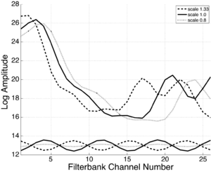
Taking the lowest 13 components has the effect of retaining the envelope of the spectrum while removing most of the harmonic structure, making the MFCCs largely invariant to pitch variability in the incoming signal. The upper lines in Figure 15 show smoothed spectra of three human /i/ vowels from speakers with different VTLs, as represented by the first 13 MFCC coefficients. To generate the smoothed spectra, the MFCCs were first calculated in the normal way, then the first 13 coefficients were retained and the inverse DCT of these coefficients was taken. The MFCC feature vector clearly contains a distinctive formant pattern: the information that the vowel is an /i/ in all three cases.

The MFCC spectrum also contains information about the relative length of the speakers’ vocal tract in the position of the spectrum along the channel dimension. The MFCC representation is not invariant to variability in source size, which shows up as the shift of the spectrum on a logarithmic scale like the ERB scale. The cosines associated with the 8th coefficient of the three feature vectors are shown in the lower part of Figure 15. Since the DCT basis functions are cosines, they cannot change phase and are all constrained to have a maximum at zero. Clearly the optimal way for the basis functions to change in response to a shift of the spectrum would be to retain the same amplitude, and to shift by changing their phase. Since this behaviour is not possible, the amplitudes of the components have to change as the source size changes, and they do so non-monotonically.

The problem remains that the individual cepstral coefficients all contain a mixture of both vowel-type and VTL information. Performing a DCT, where only the magnitude and not the phase of the basis functions may vary, means that they are specifically prohibited from shifting with acoustic scale. The maxima of a given cosine fit a set of formant peaks for a vowel with a given VTL, but they cannot shift to follow the formant peak pattern as it shifts with VTL. For example, the lower section of Figure 15 shows that the magnitude of the 8th coefficient changes markedly with changes in VTL.

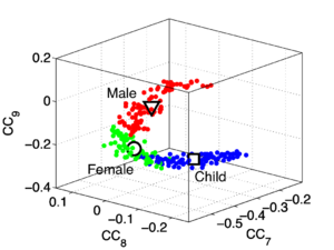
The problem that MFCC feature vectors pose for the recogniser is illustrated in Figure 16 (redrawn from an original figure by Christian Feldbauer, and published in Patterson, Walters, Monaghan, Feldbauer and Irino (2010)). It shows the feature space formed by the 7th, 8th, and 9th cepstral coefficients for the vowel /i/ as VTL varies over the range of human lengths. Whereas the mel-frequency spectrum shifts in an approximately linear way as VTL increases with height, the magnitudes of the individual components change in a nonlinear way. The square, circle and triangle show average values for children, women and men respectively. A recogniser trained on the /i/ vowels of a group of adult males (in the region of the triangle) is unlikely to recognise the /i/ of a woman (in the region of the circle) or the /i/ of a child (in the region of the square) as being within the cluster it learned for /i/.

Scale-shift invariant representations

Benzeghiba et al. (2007) cite a number of alternative approaches to VTLN. Most of these approaches involve some form of warping of the frequency axis or the normalisation of the frequency spectrum to some 'canonical' speaker. Alternatively, Mertins and Rademacher (2005) present a VTL-independent feature based on the cross-correlation between adjacent frames of the spectrum. The system relies on the fact that the spectral centroid of an utterance will shift as a function of vocal tract length. Cross-correlating adjacent frames will tend to 'normalise' the spectrum (while blurring it), shifting the spectrum of a frame towards the overall spectral centroid and thus giving a signal which is more resistant to shifts in VTL. The features developed in this section are designed to summarise the speech information directly in a shift-independent manner, rather than distorting the tonotopic axis of the auditory model, which is the equivalent of the spectral axis in MFCC systems. In the system described here, the information in the cochleogram is summarised by its spectral profile and fitted with a mixture of Gaussians, and several constraints are applied to ensure that they fit only large and well-spaced spectral peaks. As a result, a shift in VTL simply corresponds to a shift of the centres of the Gaussian functions as a group.

Features for size-independent speech recognition

Note:

Parts of the work in this section was performed in collaboration with Jessica J. M. Monaghan and Christian Feldbauer. The collaborative work was presented in Monaghan, Feldbauer, Walters and Patterson (2008)

Introduction

As demonstrated above, the standard MFCC features normally used for speech recognition have a problem in that they do not vary in an easily predictable way with speaker VTL. Therefore, we would expect that a standard speech recognition system based on MFCCs would perform poorly when trained on a single speaker (or small group of speakers with similar VTLs), and then tested on a speaker with a different VTL.

Turner, Walters and Patterson (2004) demonstrated that around 90% of the variability in the formant structure of vowels of different speakers is due to VTL changes, so speaker-independent speech recognition is, to a good first approximation, equivalent to VTL-independent speech recognition. Furthermore, Turner, Walters, Monaghan and Patterson (2009) demonstrated that formant scaling is linear, meaning that changes in VTL correspond to simple shifts of the spectrum on a logarithmic scale. Therefore, if it is possible to find a representation of the spectrum that is, to some degree, invariant to shifts in the spectral dimension, then this representation should perform better than the MFCCs when used as a feature for a size-invariant speech recognition system.

In order to demonstrate these effects, we set up a hidden Markov model (HMM) syllable recognition system based on HTK (the HMM toolkit), a standard tool for speech recognition research. The syllable recogniser was set up to use either MFCCs, or features generated from a cochlear filterbank. The training data were human syllables from a single talker, and the test data were the same human syllables scaled using STRAIGHT to a range of VTL and GPR combinations. In what follows, the word ‘speaker’ refers to utterances resynthesised from the single talker but with theoretical vocal-tract length chosen from a range of values. Features that are more robust to changes in the source size will give better performance when trained on data from a speaker of one size, and then tested on a range of speakers of different sizes.

The VTL-invariant features developed here also serve as a baseline system for a set of features developed in chapter 4, where the auditory model is extended to incorporate the noise-robustness exhibited by the stabilised auditory image.

Scaled syllables

Figure 17 --- The spoke pattern of scaled syllables in GPR-VTL space.

A database of 185 human utterances, consisting of 180 syllables and five vowels, was used as the basis for the experiments. The database consists of five strong vowels (/a/, /e/, /i/, /o/, /u/) crossed with 6 sonorant consonants, 6 fricative consonants and 6 stop consonants to produce 90 consonant-vowel and 90 vowel-consonant pairs. In addition, the five sustained vowels are included in the set (Ives et al., 2005). STRAIGHT was used to generate 57 versions of the syllable database (referred to as ‘speakers’) in which the syllables were all transformed to have a specific combination of VTL and GPR. There was a `central' speaker with a GPR of 171.7 Hz and a VTL of approximately 15 cm, and seven speakers on each of eight spokes radiating out from the central speaker in log(GPR)-log(VTL) space as shown in Figure 17. The seven speakers along each spoke are spaced logarithmically in log(GPR)-log(VTL) space. The entire spoke pattern is rotated 12.5 degrees clockwise from the axes, ensuring that there is both a VTL change and a GPR change between any pair of stimuli. This rotation was chosen as it causes one spoke to lie parallel to the line connecting the average woman and the average man in the GPR-VTL plane. This same configuration of scaled stimuli was used by Vestergaard et al. (2009) for the evaluation of human perception of concurrent syllables.

Scale-shift invariant features

Figure 18 --Scale-shift invariant features for two scaled vowel sounds

When plotted on a logarithmic scale, such as the ERB scale used in the gammatone, dcGC and PZFC filterbanks, the formants of speech have a shape that is roughly Gaussian. Furthermore, since the bandwidth of formants increases as their centre frequency increases (Hawks and Miller, 1995), the variance of the Gaussian remains roughly the same as a function of centre frequency. Given these observations, a Gaussian mixture model (GMM) was used to summarise the information in the spectral profile of the auditory image. The spectral profile is modelled as a probability distribution, and fitted with a set of Gaussians of fixed variances. The profile is then described by its overall energy, and the means and amplitudes of the Gaussians used to fit it.

Gaussian features have previously been shown to be effective in single speaker systems (Zolfaghari et al., 2006; Stuttle and Gales, 2001), and so should provide a succinct, low-dimensional, representation of the spectral profile.

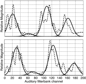
Figure 18 shows the results of fitting four Gaussians to spectral profiles for two /i/ vowels from speakers with different VTLs. There are several major concentrations of energy, the formants, in vowels. The largest three of these are fitted by three of the Gaussians. The remaining distribution is of low energy and acts as a 'spacer', encoding the presence of a spectral gap.

Expectation maximisation for Gaussian fitting

The expectation maximisation (EM) algorithm (Dempster et al., 1977) was used to fit Gaussian components to the AIM spectral profile. The EM algorithm is an iterative process which seeks to find the set of parameters for the Gaussian components which allows them to fit the spectral profile as closely as possible. The algorithm has two steps, the expectation step, in which the probability that each point in the spectral profile came from each of the current Gaussian components is calculated, and the maximisation step which updates the parameters of the Gaussian components to best reflect the estimate. These two steps are repeated until the Gaussians provide a good enough fit to the data. In order to ensure a good fit, it was necessary to constrain the standard EM algorithm in a number of ways, based on prior knowledge of the form of a vowel spectrum, and some heuristics. These modifications to the EM fitting procedure were made by Christian Feldbauer.

As discussed above, formant bandwidth increases with frequency, such that when plotted on a logarithmic scale the width remains relatively constant. For this reason, it is possible to constrain the Gaussians to have a fixed standard deviation. The optimal choice of this standard deviation was found to be around 10.7 channels (a variance of 115 channels squared) in initial experiments on a constrained set of vowel sounds. Given that the majority of energy in speech is carried in the vowels (Greenberg and Ainsworth, 2006), this approach seems reasonable as a first approximation.

The second modification introduces a 'repulsion' term between the Gaussians, which adds a penalty for too much overlap between the individual components. This is achieved by expanding and then re-normalising the conditional probabilities of the mixture components at each iteration of the EM algorithm. This expansion is according to a power-law with an exponent of 0.6. This parameter was again chosen in initial testing with vowel sounds only.

Finally, an initialisation stage was introduced distribute the Gaussians across the whole frequency range at the start of the EM process and preclude their converging on specral peaks associated with resolved harmonics of the GPR. In this step, a pair of Gaussians is first fitted to the whole spectrum using the modified EM algorithm described above. Then, the initial locations for the four Gaussians in the main fitting stage are chosen relative to the final locations of the two components in the initial fitting stage.

Calculating spectral profiles

Spectral profiles from AIM were produced by low-pass filtering the NAP to blur short-term fluctuations in its level, and then summing short sections to obtain the desired frame length. Profiles of the NAP were calculated for 20-ms frames of each syllable file in the scaled syllable corpus. The linear gammatone filterbank was used as the cochlear model, the NAP was generated by half-wave rectification and was then low-pass filtered with a second-order filter with a cutoff frequency of 100Hz. Feature vectors were generated by first applying power-law compression with an exponent of 0.8 to the profile magnitude and normalising them to sum to unity. This power-law compression was found to improve recognition accuracy in preliminary testing.

Feature vectors

Employing four Gaussian components to fit the spectral profile, and using the technique described above, there are, in total, seven degrees of freedom that can be fitted by the model: the location of the means of the four Gaussians, and the weights of three of the four Gaussians (the weight of the fourth is fixed, since the profile is normalised before fitting). In addition to these seven degrees of freedom, the energy of the profile before normalisation is also available as a further piece of information.

The weights of the Gaussians are scale-independent as they are, but the means of the Gaussians are not. The pattern of formants moves approximately as a unit on the quasi-logarithmic ERB frequency scale (see chapter 1), which means that vowel-type information will be encoded by the pattern of distances between the means of the Gaussians, providing the lowest and the highest Gaussian are allowed to move far enough to encode the scale shifts as they arise in the spectral profile. This means that we should also consider adding the three differences between the means of the Gaussian components to the feature vector. In practice, for the fairly simple task of scaled syllable recognition, it was found that four components of this set, the weights of the three Gaussians, and the total energy were enough to provide good recognition results.

In the same way as for the MFCCs, first and second difference coefficients were computed between temporally adjacent feature vectors and added to the feature vector in all cases. Thus, the length of the AIM feature vectors passed to the recogniser was 12 components, whereas it was 39 components for the MFCC feature vectors. Having feature vectors with a lower dimensionality substantially reduces the time taken to run the training and recognition algorithms in full-scale systems.

HTK for syllable recognition

Figure 19 --- Topology of a three-emitting-state HMM. The

a i j

are the transition probabilities and the

b i (o t)

are the emission probabilities.

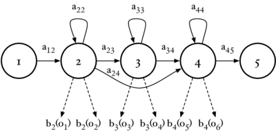
The hidden Markov model toolkit (HTK) (Young et al., 2005) was used as the machine learning system for these experiments. HTK is a research tool for investigating hidden Markov models (HMMs), and is most commonly used in speech recognition research. In an HMM speech recognition system, the speech signal is modelled as a sequence of stationary `frames' of audio which have been generated by an underlying Markov model. The frames of speech are represented as `feature vectors' -- some low-dimensional summary of a short segment of audio. A Markov model is a probabilistic finite state machine, consisting of a sequence of states, and a set of transition probabilities between those states, $a i j$ (where $i$ and $j$ are state indices). When the system is in an `emitting' state, $i$ , it will emit a given feature vector $o t$ with probability $b i (o t)$ . HTK uses a Gaussian mixture model (GMM) as a continuous density multivariate output distribution to model the continuous variables from the feature vectors. Figure 19 shows the topology of a three-state HMM.

In the case of a simple syllable recogniser, each possible syllable is represented by a single HMM. At training time, the transition probabilities and emission probability distribution for each HMM are learned.

Experiments

The models were trained on the reference speaker at the centre of the spoke pattern (Figure 17) and the eight speakers closest to the reference speakers to simulate the training of a standard, speaker-specific automatic speech recognition system.

The complete set of audio for all syllables and all speakers consists of 10,260 audio clips, each of around 600ms. All the audio was converted to both MFCCs and scale-shift invariant features. The MFCCs were produced using HTK's HCopy command and the scale-shift invariant features were produced using AIM-C, employing modules for the gammatone filterbank, the NAP and the Gaussian fitting procedure.

In training, the parameters of each syllable model were estimated from the nine speakers in the training set. The recognisers were then tested on the complete set of scaled speakers without further training. The voices used in training were also added to the test set for completeness, but reported results are for the standard test set only.

The HMM topology, number of components in the output distribution, and number of training iterations of the HMM all contribute to the overall recognition performance. In order to optimise these variables, and to provide a suitable comparison between systems, an exhaustive search was performed over all these variables for each of the two datasets. HMM topologies from 1 to 6 emitting states, and from 1 to 7 Gaussians in the output distribution were tested. 15 training iterations were performed, and every configuration was tested after each training iteration from 5 to 15.

Results

Tuning HMM parameters

Overall recognition performance was tested over the full range of HMM configurations described above. Recognition performance is reported as the percentage of the test syllables which were correctly identified by the recogniser. Performance of the HMM-based recogniser on the two sets of features was markedly different, leading to overall differences in recognition rate which were in general much larger than those due to the changes in the HMM parameters. Optimum performance, of 72.3% syllable accuracy on the MFCC features, was achieved with an HMM with 2 emitting states and with 4 components in the output distribution. This performance was achieved after 15 iterations of the training algorithm. For the AIM features, the optimum recognition performance was 93.2% across all syllables using an HMM with 2 emitting states, 6 output distribution components and after 10 training iterations. Figure 20 shows the overall syllable recognition rate for the MFCCs and AIM features respectively as a function of the various HMM parameters. For the MFCCs, the performance after 2 more training iterations for all HMM parameters shown in the plot is between 64% and 72.3%. For the same set of parameters with the AIM features, performance is between 78% and 93.2%. Performance is consistently better for the AIM features across all tested HMM configurations. (In addition to the HMM configurations shown in this graph, odd-numbered values of the HMM parameters were also tried but, for simplicity of presentation, they are not plotted here. These results cluster in the same way.)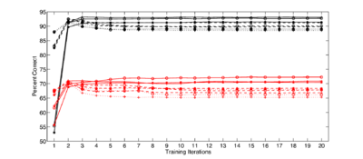

Figure 20 --- Performance of HMMs with varying parameters, trained using AIM features (black) and MFCCs (red). The vertical axis shows overall recognition performance. The horizontal axis shows the number of HMM training iterations. Solid lines denote HMMs with 2 emitting states, dashed lines 4 emitting states and dotted lines 6 emitting states. Stars show performance with 2 Gaussian components in the output distribution, circles are for 4 components and plus symbols show performance with 6 components).

Feature comparison

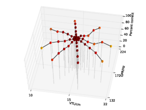
For the AIM features, 92.6% accuracy was achieved with the 2 emitting state, 4 component HMM model after 15 training iterations. Since this performance is almost at the ceiling for the AIM features, and the same HMM parameters lead to optimal performance for the MFCC features, all further comparisons are made using recognition results for an HMM with these parameters. This allows for a direct comparison of the features using an otherwise identical recognition system. Recognition performance as a function of speaker GPR and VTL for the MFCC features is plotted in Figure 21, and recognition performance for the AIM features is plotted in Figure 22.

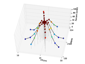
Figure 21 --- Recognition results for the MFCC features for a 2-emitting-state HMM with 4 output distribution components after 15 training iterations.

Figure 22 --- Recognition results for the AIM features for a 2 emitting-state HMM with 4 output distribution components after 15 training iterations.

For both feature types, recognition performance is best for the central speakers around the training voices, and becomes worse as the speakers change in VTL and GPR from the training region. However, the pattern of the reduction in performance is markedly different between the two feature types. Overall recognition performance with the MFCC feature vectors was 70.9% correct. Performance holds up well along the spokes where VTL does not vary much from that of the reference speaker. This subset of the results illustrates the standard finding that MFCCs are robust to changes in GPR, primarily because the process of extracting MFCCs eliminates most of the GPR information from the features. However, as VTL varies further from the training values, performance degrades rapidly, particularly on the spokes with large VTL change, where recognition falls to a minimum of 3.2% for the extreme VTL values. This provides a practical demonstration of the known lack of robustness to changes in VTL associated with the lack of scale-shift covariance in MFCCs.

Overall recognition performance with the auditory feature vectors was 92.6%. As with the MFCCs, performance remains high along the spokes associated with major changes in GPR. However, performance along all of the spokes also remains near ceiling, and only drops off significantly at the extremes of VTL. Recognition accuracy both at the longest and the shortest VTL was 71.9%, which compares with 3.2% and 4.9% respectively in the MFCC case.

Comparison with standard VTLN

Figure 23 --- Warping the frequency axis for VTLN. The warping factor

α

controls the gradient of the centre part of the line.

f L

and

f H

control the lower and upper 'break' points of the line respectively, such that the full range of input frequencies are mapped to the full range of output frequencies. This figure is redrawn from the HTK book (Young et al., 2005).

The standard approach to VTLN involves applying a piecewise linear warping to the frequency axis of the mel filterbank before the MFCC coefficients are computed. With the correct per-speaker choice of warp factor, it is possible to map the format patterns for different VTLs to the same pattern. However, in order for this method to be successful, the correct warping factor must first be found and MFCC features must be computed using this factor. In order to do this, it is usual to use a two-pass recognition process where basic recognition is performed on an un-normalised version of the features in the first pass, and then this information is used to help find the optimal warping factor for the second pass of processing.

Figure 23 shows the warping scheme used by HTK's HCopy tool when computing MFCCs. A frequency warping factor, $α$ , controls the gradient of the central part of the line, and two parameters control the upper and lower frequencies bounding this line. Outside this range the gradient is such that DC input maps to DC output, and input at the Nyquist frequency maps to output at that same frequency.

If a VTLN system performs optimally, then it should be possible to infer the ideal warp factor for every speaker at test time. In the case of the syllables database the optimal frequency warping factor is already known, since the input syllables are themselves scaled. From the original VTL values, it is easily possible to calculate the optimal warp factors and so it is possible to simulate the effect of a perfect VTLN preprocessor.

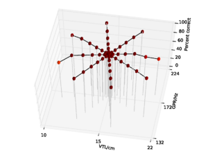
Figure 24 --- Recognition results for the syllables database using optimally VTL-warped MFCC features. Performance is consistently good across the whole range of speakers because prior information about the VTL of the speaker is provided when computing the features.

These optimal factors were calculated for the syllables database, and per-speaker MFCC features were generated. $f L$ was set at 10Hz and $f H$ was set at 10500Hz, to encompass almost the full range of frequencies when a 22kHz sampling rate is used for the input. The scaled MFCC features were then used to train a standard 2 emitting-state, 4 mixture-component HMM. The normal training set of the central speakers was used. Recognition performance was 99.0% across the whole test set, with the most errors being made on the speaker with the shortest VTL, where performance fell to 84.9%. Figure 24 shows the results for these optimally-warped features as a function of VTL and GPR. From this result we see that, if it is possible to perform good VTLN, then the MFCCs perform very well indeed. In practice such a system would require the computation of MFCCs with a number of warping factors for each utterance; the recognition system would then attempt to find the warping of the features which minimises the recognition error.

Comparison of computational complexity

While the AIM Gaussian mixture features provide better recognition performance than standard MFCC features, they are considerably more costly to compute. To compute the AIM features for the entire scaled syllables database of around 10,000 600ms sounds (100 minutes of audio) takes approximately 160 minutes of CPU time on a modern, single-core computer. By comparison, it takes just 5 minutes to compute the MFCC features using the same system, so the AIM features are approximately 32 times more costly to compute. However, there are several factors that need to be taken into account when considering whether or not this has a significant impact on the usefulness of the features. Firstly, the MFCCs were computed using HCopy, which has been progressively optimised over years of use; AIM-C, by contrast, is relatively fast as auditory models go, but it has not yet been optimised for speech recognition. Furthermore, in order for a VTLN system to be useful, warped MFCCs would have to be calculated for a range of warping factors. Welling et al. (2002) applied a total of 13 different VTL warpings to each utterance to assess their VTLN system. If this many warpings are required for good performance, then the computational cost of the AIM features becomes more competitive. It is also the case that AIM's VTL-invariant features make it possible to reduce the complexity of the recognition system, and training times.

Comparison with wide-range training

Performance of the standard MFCC features was low when the recognizer was trained on only the central speakers. This result is expected, since the MFCCs are not scale-invariant. However, in real speech recognition systems, it may be possible to train on a range of speakers. It is possible to compare performance of the MFCCs and AIM features on a wider range of speakers by training the HMM using the speakers from the outer end of each spoke in the spoke pattern.

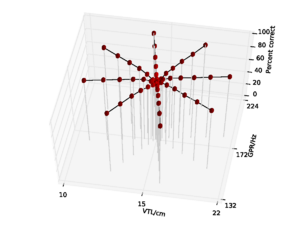
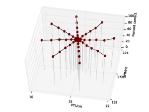
Figure 25 --- Recognition results for MFCC features when trained on the extreme outer speaker on each spoke of the pattern. Performance is highest immediately around the training data, and falls slightly further from the training speaker, reaching a low of 93.0%.

Figure 26 --- Recognition results for the VTL-invariant AIM features when trained on the extreme outer speaker on each spoke of the pattern. Performance is highest immediately around the training data, and falls slightly further from the training speaker, reaching a low of 97.3%.

The syllable recognition experiments were repeated using these speakers for training, giving a wide variety of different VTL-GPR combinations to train on. The results for the VTL-invariant features are shown in Figure 26 and the results for MFCCs are shown in Figure 25. For the AIM features, performance was 98.4% and for the MFCC features performance was 97.3%. In both cases, performance is best closest to the training speakers, and then 'sags' slightly in the middle of the range, at the largest distance from the training data. For the MFCC features, that sag is slightly more pronounced, with recognition performance falling to 93.0% around the central speakers. By contrast performance only falls to 97.3% for the AIM features.

For completeness, the MFCC features with optimal VTLN were used with the same train/test configuration. In this case, recognition performance was 100% correct across the entire space. The results are shown in Figure 27.

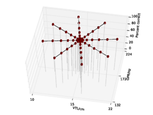
Figure 27 --- Recognition results for MFCC features with optimal vocal-tract length normalisation when trained on the extreme outer speaker on each spoke of the pattern. Performance is perfect across all speakers.

This result suggests that the HMM used in these experiments is more than capable of learning the variability of the database, so if there is a reasonable range of training data then there may be little utility in pre-warping the features. This suggests that when the training data for a multi-speaker recognition is limited to a small number of speakers, it would probably prove useful to begin by warping the VTL and GPR of the speakers to the range of values likely to be encountered by the system, and then train on all the warped utterances as well as the original utterances.

Conclusions

This chapter focuses on the observation that human speech recognition is highly robust to changes in VTL and GPR, and the discovery that a GMM can be used to extract features that are largely invariant to changes in VTL and GPR from the output of a common auditory filterbank. These auditory features were compared to standard MFCC features using a simple syllable recognition task and a database of syllables scaled over a large range of both GPR and VTL values. The scale-invariant features were found to be considerably more robust to changes in speaker VTL than MFCCs, and equally robust to changes in GPR. The experiment focuses attention on this well known deficiency in MFCC features. The success of the recognition system with VTL-invariant features appears to depend almost entirely on the features themselves, rather than the recognition system used to compare the two forms of features. Changing the parameters of the HMM recognition system has only a minor effect on performance compared with changing the features themselves. However, when scaled training data are made available to the recognition system, performance with MFCCs becomes comparable to that with the VTL-invariant features, as might be expected.

A procedure to perform VTLN on MFCCs (Welling et al., 2002) was evaluated using the scaled-syllable database of Ives and Patterson (2008). Since the original scaling factors are known it is possible to perform 'optimal' VTL warping when generating MFCC features for use with the recognizer, and so determine the best performance attainable with a VTLN system. With this optimal VTLN, recognition performance with MFCCs is extremely good. This validates the theory behind this form of VTLN, however, it should be noted that this form of VTLN is computationally expensive, and good performance can only be achieved if the recognition system correctly identifies the precise scaling factor for every speaker. The VTL-invariant AIM features currently take around 30 times more computing power to calculate than the MFCC features, but they provide a representation which does not require any further processing to be used in a standard speech recogniser. By contrast for VTLN, MFCC features would have to be computed with a range of around 10 different VTL warpings and then be passed to a more complex recognition system in order to be useful.

The scale-shift "invariant" features derived with AIM exhibit some residual sensitivity to change in VTL. Since it affects only the extreme VTL conditions, it seems likely that the sensitivity is due to edge effects at the Gaussian fitting stage. That is, when a formant occurs near the edge of the spectrum, the tail of the Gaussian used to fit the formant prevents it from shifting sufficiently to centre the Gaussian on the formant. If this proves to be the reason, it suggests that performance is not limited by the underlying auditory representation but rather by a limitation in the feature extraction process.

The scale-shift invariant features described in this chapter were generated from the output of an auditory filterbank, but beyond this, the processing bears little resemblance to that performed in the auditory system. Rather the features demonstrate a macroscopic property of the auditory system. In the following chapter, I look in detail at a proposed model of the processing performed in the early stages of the auditory pathway. The auditory image model (AIM) describes a process of strobed temporal integration in which signals from the cochlea are 'stabilised' with respect to the pulses in the input sound in order to generate a stabilised auditory image (SAI), which changes over time. In chapter 3, I concentrate particularly on systems for strobe point identification. One hypothesised benefit of AIM is that the SAIs which it produces are more robust to interfering noise than simple spectral representations. In chapter 4, the feature-generation system developed in this chapter is extended for use with the SAI representations developed in chapter 3. The procedure developed in the current chapter for comparing auditory features with MFCCs is used in chapter 4 to compare the performance supported by various SAI-based representations with the performance of MFCCs as the speech signal sinks into background noise.

Strobes and Stabilised Auditory Images

The last chapter introduced a feature representation based on the smoothed output from a simulation of the cochlea and a simple hair-cell model. The signal was temporally averaged over a short window by means of a low-pass filter. Strobed temporal integration, leading to a stabilised auditory image (SAI), is an alternative, more complex, system for processing the signal leaving the cochlea. Strobe points are identified in each channel of the filterbank output, and these points act as triggers for a temporal integration process in which shifted copies of the signal are overlaid on one another.

Since strobe points tend to occur at or near the pulses in a pulse-resonance sound, representing a signal containing a pulse-resonance sound as an SAI will tend to accentuate the periodic, pulse-resonance components of a signal relative to any background noise. Noise-robustness is an extremely useful property in any machine hearing system, and so we wanted to incorporate the inherent noise-robustness of the SAI into our auditory model. In this chapter, existing mechanisms for strobed temporal integration are assessed and compared, and the theoretical basis of this mode of temporal integration is investigated in an effort to identify a simple criterion for optimal strobe generation. The goal was to create a stabilised auditory image for a noise-robust machine hearing system.

Strobe finding in AIM

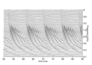
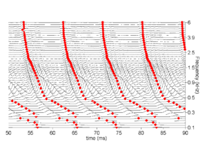
Figure 28 -- Neural activity pattern for a short segment of the vowel /a/.

Figure 29 -- Strobe points detected for the NAP shown in Figure 28

In the auditory image model, stabilised auditory images are produced by strobed temporal integration. An image is built up by repeatedly adding sections of a NAP signal to a buffer. Each time a `significant' event or `strobe' occurs in the signal, the process restarts, adding the signal following the strobe to the buffer, starting at zero. Strobed temporal integration is central to the production of SAIs.

When processing a pulse-resonance communication sound in AIM, it is desirable that the strobe points should fall at points in the NAP signal which were caused by a pulse in the original sound. When this occurs, the resonances following each pulse are added exactly in phase in the auditory image, such that the resonances following each vertical ridge in the image resemble as closely as possible the original resonances in the sound. However, this requirement is somewhat ambiguous because the response of the auditory filterbank to a pulse is not a single peak, but a series of peaks within an envelope.

In practice, it is not necessary for the strobe finding to be perfectly accurate in order that a good SAI be built up from a pulse-resonance sound. The exact choice of which peak of the filter's impulse response to strobe on does not make a significant difference to the auditory image that is produced, and there does not have to be exactly one strobe for each glottal cycle. However, the closer that it is possible to get these requirements, the more accurate the SAI will be. It is desirable that there should be roughly one strobe per pulse, that the choice of strobe points should be reasonably consistent across channels and across pulses and that strobe timing should not be affected too greatly by the exact form of the resonance following each pulse.

Figure 28 shows the neural activity pattern (NAP) from a short segment of an /a/ vowel. Figure 29 shows a set of strobe points on that NAP. There is exactly one strobe point per cycle in each channel, and the strobe points occur consistently at the peak of the envelope in each channel, so in some sense the algorithm applied here has found the optimal set of strobe points for this signal.

Relationship to pitch detection

Strobe-point detection is, in some respects, a similar process to pitch determination of a time-domain signal (albeit a signal which may have been passed through a nonlinear filter). Computational auditory models which can extract the pitch of complex sounds (see, for example, Brown and Cooke, 1994) must, necessarily, integrate over a few cycles of the pitch period to get a result. Robinson and Patterson (1995) showed that humans take between four and eight cycles of the waveform to extract useful pitch information, but the information required to identify a vowel can be extracted from a single cycle of the wave, and so it is unlikely that long-term pitch extraction can play a direct role in timbre extraction. However, the task of instantaneous detection of peaks in the time-domain waveform is still related to that of pitch detection in the time domain.

There is a rich literature on the subject of pitch detection in time-domain signals and Hess (1983) provides an excellent overview of the state of the field at that time.

Hess identifies four significant features from which periodicity in a signal can be derived in the time domain. The first two of these features are:

The presence of a fundamental harmonic.
A structural pattern which repeats from period to period.

The second pair of features is derived from the linear model of speech production, which is the production mechanism for pulse-resonance communication sounds described in chapter 1. Using this model, Hess identifies the following:

High amplitudes at the start of a period and low amplitudes at the end, since the vocal tract can be assumed to be a linear passive system whose impulse response consists of exponentially decaying sinusoids (Fant, 1960).
Discontinuities in the signal or its derivatives at the instants where individual pulses occur.

The pitch determination algorithms reviewed by Hess are, of course, all based on analysis of the original waveform, rather than the output of an auditory filterbank, but the principles in each case are similar, and the temporal features which he describes translate to the filtered case.

The majority of algorithms for strobe finding employed in AIM rely on the third of Hess's features to perform their classification of strobe points. When a pulse excites resonances which decay with a finite time constant, an exponential threshold which decays more slowly than the resonance can be applied to the signal to `follow' the decaying resonances. When this threshold is exceeded, a pulse is deemed to have occurred. This simple idea has been proposed and implemented many times; indeed Hess cites over 20 references to proposals for analogue versions of this scheme dating from 1949 to 1977.

In this section, I review some of the basic properties of the auditory filterbank and human vocalisations to help derive the correct constraints for a strobing scheme that is in some sense optimal for a given filterbank and expected class of signals.

Thresholding

Figure 30 --- 'Peak' strobing criterion -- strobes are issued on all local maxima of the NAP.

Figure 31 --- 'Temporal shadow' strobing criterion -- strobes are issued on each local maximum if it exceeds a decaying threshold.

Figure 32 --- 'Temporal shadow with timeout' strobing criterion -- strobes are issued as in the `temporal shadow' case, but there is a 5ms timeout imposed after each strobe which prevents another strobe from occurring in that time.

Figure 33 --- `Parabola' strobe criterion -- here the timeout is encoded explicitly as a parabola that can `jump over' intervening peaks.

Figure 34 --- `Bunt' criterion -- after each strobe, the threshold jumps up by a random amount

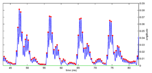
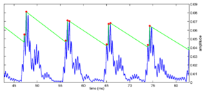
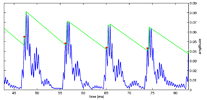
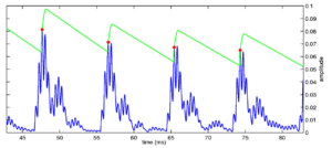
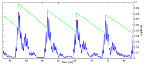
The basic mode of operation of strobing systems is to place a decaying threshold on the incoming NAP signal. The threshold starts off at zero activity, and it is updated constantly. When the level of an incoming NAP peak exceeds the threshold, the threshold is raised to that level, and a strobe may be issued at that time. After the peak, the threshold decays in some way with time, and any NAP peaks which are under the threshold are ignored. A strobe can be issued on every NAP peak which is above the threshold, or only on a subset of those peaks, based on some other criteria. The versions of AIM software over the years have, for the most part, used variations on this basic scheme as the basis of their strobing systems. The major differences between the strobing schemes are in the form of the threshold that is used. These various criteria are presented in the documentation for AIM1992 and AIM-MAT, and I present the basics of each system below.

Various strobe detection schemes have been added to AIM over the years. The initial version of AIM, AIM92, was written by John Holdsworth and Mike Allerhand, with contributions from Christian Giguere and Michael Akeroyd. This version included the 'peak', 'temporal shadow' and 'local maximum' strobe criteria. AIM-MAT, which was released in 2003, was written by Stefan Bleeck. This version added the 'bunt' and 'parabola' mechanisms in addition to the strobe criteria from AIM92.

Figure 30, Figure 31, Figure 32, Figure 33 and Figure 34 show the form of threshold in each of the various strobe algorithms employed in AIM1992 and AIM-MAT. The simplest strobe criterion (not shown here) is just to issue a strobe point at every nonzero point in the NAP. This leads to a representation which is very similar to a correlogram. The next simplest is to issue a strobe on each local maximum in the NAP --- the `peak' strobe criterion. In this case as well, much of the asymmetry in the NAP is not preserved in the auditory image generated, leaving a representation that looks similar to a correlogram, once again. The benefit of this method, however, is a significant reduction in the rate of strobe points, and so a similar reduction in the computational complexity of the SAI generation process. This computational efficiency is one of the major practical benefits of strobed temporal integration above autocorrelation.

The next, more complex, systems add the decaying threshold to the NAP to decide whether a strobe should be issued or not. In applying a decaying threshold, some prior knowledge of the form of the information in the NAP is applied to the processing. By applying this threshold, the assumption is that the input sound has a pulse-resonance structure with strong onsets and decaying resonances. As we have seen, this is an entirely reasonable assumption to make about the sounds encountered in everyday life (although it is always possible to construct `pathological' stimuli that break this assumption, for example the ramped sounds presented below).

The `temporal shadow' criterion is the simplest of these thresholded criteria. In this case, a decaying threshold is placed on the signal. This threshold is reset to the level of the NAP at the time when a strobe is issued, and then decays linearly such that it is zero after a predetermined time period. However, this system does not take into account the finite rise time of the auditory filter and issues strobes on all NAP peaks within the rising edge of envelope maxima.

In order to combat this, a timeout can be added which prevents the system from issuing a strobe in a short window after a previous strobe point. This means that the first peak in the rising edge of a new pulse is the strobe point, and as long as the rise time of the filter's impulse response is short enough, no more strobes will be issued on this peak. In this case, the strobe threshold is reset on each strobe candidate, rather than each strobe point. The timeout, however, has the effect of suppressing strobe points on the local maximum of the envelope. The system will issue a strobe point on the first NAP peak in a rising edge, and the timeout will prevent subsequent strobes.

Further variations come in the form of the 'parabola' and 'bunt' strobe criteria found in the sf2003 module of AIM-MAT. In these systems, the timeout is more explicitly encoded in the threshold. In the 'parabola' case, the threshold is 'thrown' up from a strobe peak in a parabolic shape. The parabola is then truncated after some period of time and the threshold then decays linearly. In the 'bunt' case, the threshold jumps up by a random amount after a strobe point and then falls linearly from its new maximum.

In all these cases, the designers were implicitly adding more prior information about their knowledge of the form of the signal emerging from the auditory filterbank, and attempting to tailor the strobe criterion to that form. Later in this chapter, I attempt to place these implicit constraints on a firmer theoretical basis in order to choose the best parameters of a strobing scheme in a principled way.

Windowing

An alternative simple strobe detection system was developed by Dick Lyon for use in the sound effects ranking experiments described in chapter 6. In this system, the signal in each channel is multiplied pointwise by a windowing function. The maximum point in the windowed signal is the strobe point. The window is then shifted by 4ms and the process is repeated. The window used is an inverted parabola of 40ms width. Thus, there is guaranteed to be an average of one strobe point every 4ms, but it is possible for multiple strobes to occur at one point in the signal, since the windows overlap. The performance of this system is evaluated along with that of the other systems later in this chapter.

Look-ahead

The major distinction between different models of strobing is whether or not a model needs to look at the signal beyond a point in time in order to classify that point as a strobe or not. In a causal system with no delay, a NAP peak may only be classified as a strobe on the basis of the information in the NAP up to and including that point; that is, strobe points may not be identified retrospectively. Any system that relies on positively identifying NAP peaks cannot have zero delay since identification of a turning point requires knowing the value of the subsequent sample.

If a process akin to strobed temporal integration is performed on the auditory signals in the brain, then strobe detection must occur with only a small delay of the order of a few milliseconds, as strobe points must be identified and acted upon without any temporal integration. If any temporal integration was required to perform strobe detection, then the main benefit of strobed temporal integration would be lost, and one might as well deal with more advanced pitch detection algorithms.

The various previously existing strobe finding algorithms described above require either simple identification of NAP peaks or a short delay of a few milliseconds before positively identifying a NAP peak as a strobe, apart from the Lyon parabola system, which may look up to 40ms ahead. The main system which I develop here is a variant on these previously existing systems, and also requires a delay of up to six milliseconds before positively identifying strobe peaks. Delays of the order of 10ms at this stage of the system are entirely reasonable from the point of view of auditory perception.

As an additional example, I present a strobe detection system that processes whole sections of the NAP across multiple channels. In this case it is necessary to look ahead on the order of 20-30ms in order to issue strobes. While this approach is reasonable in a computational system, it may bear less resemblance to the processing performed by the auditory system.

Noises and damped/ramped sounds

One major concern for a strobing system is that it should be able to `degrade gracefully' in the presence of a sound that is not of the type that it is optimised to deal with. In the case of noises, strobe points can occur at random, but the rate of strobes should be high enough that an SAI is still built up.

Time-reversed pulse-resonance sounds present an interesting problem for a system that is optimised for normal pulse-resonance communication sounds. These 'ramped' stimuli are characterised by an exponentially increasing envelope that is suddenly truncated and falls to zero. Figure 35 shows an example of the waveform for an idealised ramped sound, and Figure 36 shows the equivalent damped sound. Ramped sounds are perceived differently by the listener to the equivalent damped sounds, and the SAI produced by these sounds should retain the asymmetry seen in the NAP for each sound (Patterson, 1994a; Patterson, 1994b).

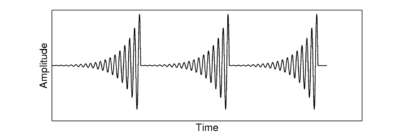
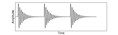
Figure 35 -- A 'ramped' stimulus is a time-reversed pulse-resonance sound. The slow onset can confuse strobe detection systems.

Figure 36 -- A 'damped' stimulus has the form of a normal pulse-resonance sound.

A simple strobe criterion like the temporal shadow method will end up strobing on every peak of the rising envelope, producing a highly symmetrical SAI for a very asymmetrical stimulus. Therefore, various modifications to the strobing system were suggested to deal with this class of stimulus. The simplest approach is to wait for some period of time before classifying a potential strobe peak as a strobe point. Such systems look ahead to see if there is a larger peak within some fixed time after the current candidate. An alternative approach is to have a strobe `lockout' that occurs after a strobe is issued, that prevents the system from issuing a strobe for some fixed period of time.

Cross-channel constraints

So far, all the strobing systems discussed have not made any use of the obvious constraints between channels. If a pulse-resonance sound hits a filterbank, then the pulse, which is by its very nature broadband, will excite channels at a whole range of frequencies. Indeed, unless the stimulus has been heavily bandpass-filtered, it will have a significant effect across the whole filterbank. It seems an obvious idea, then, to look across multiple frequency channels when trying to detect strobe points.

A set of criteria for good strobe detection

Having discussed the various desirable features of a strobe system, we can draw up a set of criteria for a good strobing system that is both computationally efficient and physiologically plausible:

Strobes should be issued on peaks of the NAP only.
For pulse-resonance sounds, strobes should be issued at a peak of the NAP that corresponds to a pulse in the input sound.
In sounds with a repeating pulse-resonance structure, only one strobe should be issued for each cycle, in each channel.
Strobes should be consistently issued on the same NAP peak within a cycle.
NAP peaks should be identified as strobes within a few milliseconds of entering the processing system.

Choosing the correct threshold

The initial problem is that of identifying the points in time at which glottal pulses occurred in a human vocalisation, given the output of an auditory filterbank excited by that vocalisation. This problem is known as event detection. Initially we deal with the simple case of a single speaker with no background noise as the input sound, and then the analysis is extended to cope with the case of a single speaker in noise, and then to multiple speakers in noise.

This process is simply a formalisation of the heuristic approach taken in the design of previous strobe detection systems. In all the systems discussed above there is an implicit assumption about the form of the sound that the system is dealing with. Event detection in the output of the auditory filterbank is informed by both the characteristics of the filterbank itself, and the characteristics of the class of sounds expected as input to that filterbank. The filterbank impulse response and the impulse response of the human vocal tract are similar in form; the form of human vocal resonances is that of any physical resonant system which is excited by pulsive excitation. This knowledge of the system can be used to constrain the problem in a way which gives reasonable event-detection behaviour for normal, physically-realisable, inputs and `degrades gracefully' in the case of unusual inputs so that in the worst case the system simply acts as a spectrum analyser.

In this section, I use the gammatone as an example filterbank. I use the characteristics of the gammatone itself, and a simple model of pulse-resonance sounds, to derive some constraints on the signal in each channel of the NAP. These constraints are then used to choose parameters for a system that performs dynamic thresholding of the signal, as with previous schemes. It requires a small `look ahead' over 10-15ms of the stimulus (and does not perform any cross-channel integration).

Additionally, I present a system which strongly enforces cross-channel constraints to infer the original pulse times in the stimulus (but which is less computationally efficient and which requires a greater 'look-ahead' time).

Filterbank and vocal tract impulse responses

For this analysis, it is assumed that the auditory filter is a simple gammatone or gammachirp filter, without any compression built in. This means that the filter has a known envelope of the form 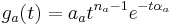$g_a(t) = a_at^{n_a-1}e^{-t\alpha_a}$ where the subscript $a$ refers to the fact that this is the auditory filter. The terms of this equation are as follows: $a a$ gives an overall amplitude, the $t^{n_a-1}$ gives a finite rise time and the $e^{-t\alpha_a}$ gives the decay. The time that the maximum occurs can be found by differentiating the filter envelope, and is found to be at $t = (n a - 1) / α a$ . This envelope, with a sinusoidal carrier -- a gammatone filter -- can be seen in Figure 37. The envelope of the resonance of the vocal tract is taken to be a simple damped exponential: 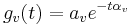$g_v(t) = a_ve^{-t\alpha_v}$ , with the $v$ referring to the vocal tract filter. We assume that the entire system of vocal tract resonator followed by auditory filter is struck by a stream of pulses which are modelled as single delta-functions 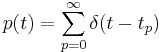$p(t)=\sum_{p=0}^\infty\delta(t-t_p)$ where the $t p$ are the pulse times. This is clearly a simplistic model of the resonances of the vocal tract, since the vocal filter cannot have an instantaneous rise time, but it will suffice for the purposes of defining constraints on the response of the system.

Figure 37 -- Envelope (blue) and impulse response (green) of the gammatone filter. This is the response of the filter to a single-pulse excitation at time

t = 0

, marked by the red cross.

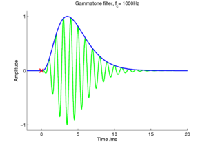
To simulate the output of the cochlea to the auditory nerve, the output of the basilar membrane is half-wave rectified. In many models, there is also a low-pass filter applied to the signal which simulates the loss of phase-locking in the hair cells at high frequencies. Since the NAP is monopolar, lowpass filtering is equivalent to leaky integration of the signal. For a first treatment of the problem, the low-pass filtering will be put aside, and signals which have simply been half-wave rectified will be considered. This class of signal is known as the Neural Activity Pattern, or NAP. Once an initial version of the model has been developed, the effect of low-pass filtering can be considered again.

Figure 38 -- Simulation of the NAP produced in the 1000Hz channel by a single pulse at time

t = 0

, marked by the red cross. The NAP maxima are marked by red dots.

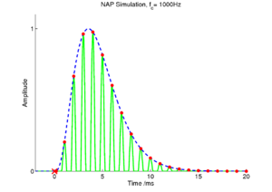
Single-pulse excitation

In the case of a single pulse exciting the filterbank, the response in a single channel is simply the impulse response shown above. This is the most simple form of excitation, and provides a good basis for developing an algorithm which will ultimately extract the timings and amplitudes of filtered pulses. Figure 38 shows a simulated NAP for the 1000Hz channel of a gammatone filterbank which has been struck by a single pulse at time $t = 0$ . This input is received as a function of time by the strobe finding mechanism. In the ideal case, the mechanism will wait as the amplitude of successive peaks gradually rises, and then fire a strobe at the top of the highest peak in the NAP. This requires the system to look ahead a certain amount of time to determine if it is indeed dealing with a rising set of peaks due to a pulse. However, the rise time of the filter is known; for a gammatone filter with a given centre frequency, the peak of the filter envelope is at $t = (n a - 1) / α a$ after the pulse, as shown above. This means that a simple constraint can be placed on the strobing system: in each channel, the system should wait for a maximum of $(n a - 1) / α a$ to see if a higher peak occurs during that time. In the high frequency channels, this time is short, but as the channel centre frequency decreases, this `look-ahead' time becomes longer.

This rise time of the filter runs from a maximum of about 15.6ms for a gammatone filter at 50Hz, to 0.83ms for a gammatone filter at 5kHz. Thus, looking forward as far as the rise time of the lowest gammatone filter requires a maximum look-ahead of about 16ms. After this time, a firm decision can be made on whether an event occurred at a certain time.

Once a strobe has occurred and the filter response starts to fall, the system can simply `follow' the decaying envelope of the filter down. Any peaks at or below the envelope of the decaying filter's response at a certain time after the strobe can be ignored. This is the system used in the decaying threshold of previous strobe finding algorithms. The decay parameters of the filter are already known: the envelope decays from a maximum at $t = (n a - 1) / α a$ following a gamma envelope.

Pulse-resonance excitation

The case of pulse-resonance excitation is an extension of the filtered pulse case. In this version, the pulse is filtered first by a resonance, and then by the auditory filter. The form of the vocal tract filter is taken to be the same as that of a gammatone filter, but with different coefficients.

The form of the envelope of this filtered response can be derived by convolving the envelopes of the impulse responses of the auditory filter and the vocal tract filter. Merely convolving the envelopes to get the combined envelope holds only when the carrier frequency of both the vocal tract and auditory filters are the same, but the on-frequency response of the filter provides an upper bound on the envelope of the response, as shown in section \ref{carrier}.

This convolution can be achieved in the Laplace domain. The Laplace transform of the function $g_a(t) = a_at^{n_a-1}e^{-t\alpha_a}$ is

$G_a(s)=a_a\frac{\Gamma(n_a)}{(s+\alpha_a)^{n_a}} ~ s>-\alpha_a$

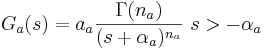
and the transform of 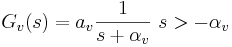$g_v(t) = a_ve^{-t\alpha_v}$ is just $G_v(s)=a_v\frac{1}{s+\alpha_v} ~ s>-\alpha_v$

To perform a time domain convolution, the Laplace transforms of the two functions are simply multiplied to give

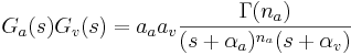
$G_a(s) G_v(s)= a_a a_v\frac{\Gamma(n_a)}{(s+\alpha_a)^{n_a}(s+\alpha_v)}$

It is possible to calculate the inverse Laplace transform explicitly for certain numerical values of the constant $n a$ (the general solution is also possible, but it is not particularly useful in this case). $n a$ is difficult to generalise over, as it appears in the power in the denominator of the function in the Laplace domain. For the simple case of a damped exponential vocal tract resonance and a standard gammatone filter ( $n a = 4$ ) an explicit case of the general equation can be found. This is:

$g_{av}(t)=\frac{6\left(e^{-\alpha_at}-e^{\alpha_vt}\right)}{(\alpha_a-\alpha_v)^4}+\frac{\left(3(\alpha_a-\alpha_v)t+t^2(\alpha_a-\alpha_v)^2+6 \right)e^{-\alpha_at}t}{(\alpha_v-\alpha_a)^3}$

which has a similar form to the gamma envelope, but with exponents of both $α a$ and $α v$ and a polynomial in $t$ rather than a single power of $t$ .

This, then, is the form of the envelope of a gammatone auditory filter struck with a decaying exponential resonance. Formant bandwidths are of the order 50-125Hz (Hawks and Miller, 1995) for frequencies up to about 3kHz. The longest decay times will be associated with the smallest formant bandwidths, so for a 50Hz formant bandwidth, $α v$ will be around $50\pi\simeq157$ . This gives an upper bound on the expected envelope of the filter response when it is driven by a formant of speech. If the minimum formant bandwidth is taken as being 50Hz, then for a gammatone filter at 1000Hz, driven by a formant at 1000Hz with a 50Hz bandwidth, the rise time goes from about 4ms to about 7ms (4 cycles to 7 cycles). This maximum rise time can be calculated in each channel in the same way.

Adding a carrier

This analysis has so far been carried out only for the envelopes of the functions involved. If the carrier is included in the calculation as well, the ensuing expression becomes even more complicated. However, since we wish only to find upper and lower bounds on the decay time of the NAP peaks in response to a damped resonance, a simple heuristic analysis will suffice.

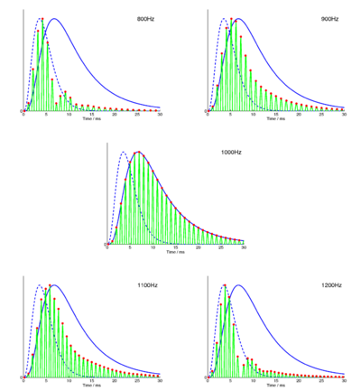
Figure 39 --- An auditory filter with a centre frequency of 1000Hz excited by a decaying resonance with a carriers of 800, 900, 1000, 1100 and 1200Hz. The envelope of the impulse response is the dotted blue line and the theoretical maximum envelope is the solid blue line.

Figure 39 shows the effect of sweeping a damped formant through the filter with a centre frequency of 1000Hz. The formant has a frequency of 800, 900, 1000, 1100 and 1200 Hz in the five panels. The maximum temporal extent of the filter envelope is when it is driven exactly on frequency; the decaying resonance has the same carrier frequency as that of the channel of the filterbank which is being observed. In the off-frequency cases, the response of the filterbank will decay faster than in the on-frequency case, and will rise to its highest value faster. On-frequency excitation is the extremal case, both for the onset and the decay characteristics of the excited filter, and so the envelopes calculated above for a gammatone filter and a damped resonance are the limit of the expected response of the auditory filters when excited with damped resonances.

Multiple pulses

The system needs to be able to identify a series of pulses followed by resonances. If the pulse rate is high enough, new pulses will interfere with the tails of previous resonances. The interaction of a given resonance decay with the onset of the next pulse makes it somewhat more difficult both to identify pulses and to track the rise and fall of vocal tract resonances.

Noise excitation

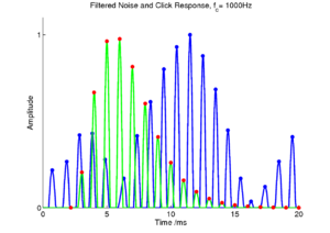
Figure 40 -- The response of the filterbank to noise (blue line) and a click (green line). The amplitudes and positions of the peaks are plotted in each case. The click in this case occurs at 2ms on the time axis. The frequency and phase of the filtered noise signal are not necessarily the same as those of the impulse response.

Another important input signal to consider is noise, as it can form part of a communication sound (for example fricatives in human speech) or be added to a signal which is to be retrieved. Figure 40 shows the effect of exciting one channel of a filterbank with Gaussian noise. Note that the output of the filter, when driven by a noise, is not necessarily at the same frequency as the filter's impulse response, and that the output frequency varies with time. In the case of bandpass filtered noise, there will be a general rise in the level of excitation for all filters in the region of the passband. A strobing system should degrade gracefully when processing any stimulus that is not a periodic, pulse-resonance signal. It should continue to issue strobes at a reasonable rate, but essentially at random. If there is no temporal structure to the input signal, then there will be no temporal structure in the SAI. In fact, the process of strobed temporal integration actively damps down noises in the SAI relative to pulse-resonance sounds. This happens because, in a noise, strobes will occur randomly, and the activity in each channel will tend to have a random phase. This means that the characteristic peaks and troughs in each SAI channel will become smeared out relative to the pattern for a pulse-resonance sound, and the overall level of activity in the SAI will be lower and the dynamic rage smaller than for a pulse-resonance sound. In this case, strobed temporal integration reverts to a form of spectrum analysis. The SAI for a noise will consist of sustained activity, proportional to the energy present in each channel.

The effect of low-pass filtering and compression

After the filterbank stage in AIM, the NAP stage simulates the response of the inner hair cells to the motion of the basilar membrane. The signal is first half-wave rectified to simulate the monopolar response of the hair cells. The loss of phase-locking at higher frequencies is then simulated with a low-pass filter, and since the signal has already been half-wave rectified at this point, this reduces to a simple leaky integrator. Loss of phase-locking is associated with the capacitance of the hair-cell synapse. The standard low-pass filter in AIM is a two-stage filter with a cutoff frequency of 1200Hz, meaning that the filter skirt is 24dB down by 4800Hz. For non-compressive filterbanks, such as the gammatone filter, compression is also added at this stage. For the gammatone, logarithmic compression is applied to the filter output before the rectification and filtering stages. To find the response of a driven filter, the envelope derived above can simply be processed in the same way as the output signal is.

A candidate system: Low-latency thresholding with constraints

Using the constraints described above, it is fairly simple to modify the parameters of some of the existing strobing systems to fulfil these constraints. A set of simple rules define the strobe system:

All points which are not local maxima are ignored.
When the signal exceeds threshold, the threshold is set to the level of the signal at that time, and that point is labelled as a strobe candidate.
The threshold decays according to the longest possible decay of the filter in that channel when struck with a damped formant.
If there are no larger strobe candidates within the rise time of the driven filter, then the candidate is labelled as a strobe.

To promote the propagation of strobes across multiple channels, an additional rule may be added:

If a strobe is known to have occurred in a higher frequency channel, then the threshold in the current channel is lowered by a set proportion for each higher channel in which a strobe occurred. The threshold is lowered in a region around the time that a strobe is expected to occur.

In practice, this system modifies the thresholding functions from previous systems to include two filter-dependent parameters: the decay rate (and trajectory), and the `look-ahead' time, which is determined by the rise time of the filter. In practice this leads to a non-causal system, where there is a short delay in classifying strobe points. The parameters of the lower-frequency channels will determine the maximum values for the look-ahead time. If some maximum look-ahead is desired, then the look-ahead can be truncated in the low-frequency channels, at the expense of accuracy.

Time constants in each channel

For each channel of the filterbank, there are three parameters of interest in the response: these are the filter centre frequency (which determines the timing between NAP peaks), the maximum rise time of a driven filter (which determines the maximum look-ahead needed before classifying a strobe point), and the slowest decay rate of a driven filter (which determines the decay rate of the threshold). Given these parameters, the `temporal shadow' strobe criterion can be updated to take into account the known properties of the filter in each channel.

To determine the time constants in each channel, the filter response derived above is processed to mimic the effect of the NAP stage on the filter output. The filter envelope derived above is correct for a gammatone filterbank, and is low-pass filtered to simulate the NAP. The other filterbanks used in AIM, the PZFC and dcGC, do not have exactly the same impulse response as the gammatone, but to a first approximation the response is similar enough to allow for improved strobing. The compression applied by these filterbanks is less aggressive than the logarithmic compression used in the gammatone, so this stage can be left out when calculating the parameters of the envelope for these filterbanks. In practice, the parameters derived and used in the experiments below are for a low-pass filtered gammatone filter with no compression in all cases. The PZFC and dcGC filternbanks are described in detail in chapter 5; the methods and main results presented here are based on the use of the gammatone filterbank, but the experimental results also include values for the compressive dcGC and PZFC filterbanks for comparison purposes.

Once the envelope has been calculated, the maximum of the envelope can be found. The time to the maximum is the filter rise time. All the parameters for the strobing system can be pre-calculated once for a given set of filterbank parameters, and then reused. The parameters to be saved are the rise time, the filter centre frequency, and the form of the decaying threshold (this is used rather than a decay rate, since the absolute amplitude of the filter response will change on the basis of the input).

Figure 41 --- The rise time,

t rise

, and decay time,

t decay

, for a gammatone filter excited by an on-frequency formant. The rise time is the time taken for the filter envelope to reach its maximum value. The decay time is the time required for the filter envelope to fall to some small proportion of its maximum height. Two possible thresholds are shown. The linear threshold passes through the peak and the next highest peak after it. The nonlinear threshold is the driven filter envelope, shifted to take account of the cases in which the highest NAP peak occurs before the maximum of the filter envelope.

Figure 42 --- Rise time of a gammatone filter driven by an on-frequency damped formant as a function of filter centre-frequency.

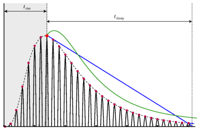
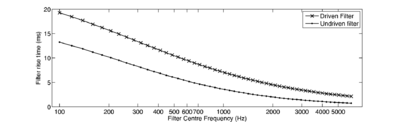
Figure 41 shows the envelope of a damped formant exciting a channel of a gammatone filter. The rise time $t rise$ is calculated in each channel. The system then waits for $t rise$ after each strobe candidate to see if any larger strobes occur in that time. If a larger NAP peak does occur, then the new peak is marked as a candidate. Once $t rise$ has passed since the first candidate, the last identified candidate is marked as the strobe point. Figure 42 shows the rise times for the channels of the standard gammatone filterbank when driven by an on-frequency formant.

There is a problem with such a simple lockout system. If the pulse-rate is faster than the lockout time, the system will not produce strobes on every pulse. To prevent the lockout from interfering with the pulse rate of the audio, a maximum lockout time can be set. This increases the chance of the system incorrectly identifying points on a rising edge in the low-frequency channels, but allows the system to strobe accurately on each peak of higher-pitched sounds. The maximum lockout is a configurable parameter. In testing it was found that good results are achieved when the strobe lockout is limited to a maximum of 6ms. This means that there is a maximum of 6ms delay between a NAP peak being identified, and being marked as a strobe point. It does, however, mean that the maximum rise time can be larger than the lockout for around two-thirds of the channels. In practice, this is not such a problem, since only a few channels will be driven strongly on-frequency at any given time. Looking at undriven filter rise times, we see that a 6ms rise time lockout only affects channels below about 450Hz. Furthermore, in the low-frequency channels there are few NAP peaks per pulse, and so the exact choice of NAP peak for strobing on is less important.

For simplicity, the temporal shadow strobe criterion (and all other previous strobe criteria) used a linearly decaying threshold from the highest NAP peak. This is simple to implement, but does not follow well the form of the actual filter decay. In initial testing of the new algorithm, it was found that strobing accuracy could be improved slightly by using a threshold that matches more closely the form of the driven filter envelope. Computationally, this approach is only slightly more expensive, but the increase is not significant because the form of the threshold in each channel can be pre-calculated and stored. Figure 43 shows the effect of applying the new constrained threshold in one channel of the filterbank. The threshold can be seen to rise a small amount before it falls. This occurs because the threshold is taken from being one NAP cycle (1/centre frequency) before the peak of the envelope, allowing for the case where the NAP peaks are out of phase with the envelope peak.

This new 'constrained thresholding' strobe detection has three major improvements over the older strobe detection systems. Firstly, all the parameters of the system are calculated from the derived envelopes of driven gammatone filters. These parameters provide an upper bound on the expected temporal characteristics of the filter response. Secondly, the 'lockout' system allows the system to follow a rising edge for a short period, and not issue a strobe point until the top of a rising edge. This means that the system will tend to issue strobe points on true local maxima of the filter envelope, rather than at the start of a rising edge (as the 'local maximum' criterion does). Finally, the form of the threshold in each channel is pre-calculated to follow the form of the decaying envelope of a driven filter in that channel. This threshold follows the real envelope of the NAP more closely than a linear threshold. The system, as described above, was implemented in AIM-MAT, and it is tested in the experiments below. Figure 44 shows the effect of running the system on a pulse train input with an 8ms interval between pulses.

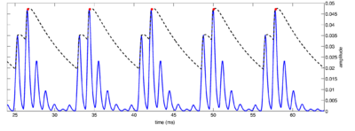
Figure 43 --- The constrained threshold system at work in a single channel. Notable features are the suppression of strobe points on the rising edge of the filter response and the non-linear decaying threshold.

Figure 44 --- Strobes detected by the constrained threshold strobe detection system for a pulse train with an 8ms interval.

A candidate system: Event-time back-projection

Given knowledge of the rise time and decay characteristics of the filter, it is possible to make an estimate of when an event occurred based on the amplitudes and timings of consecutive peaks of the NAP. This algorithm calculates a distance measure from the impulse response of the system to the current state at every point in time. This has the effect of tying together the responses of all channels and determining a single strobe time across the entire filterbank. The system marks the presence of a pulse in all channels, even if it is masked by other energy in some of those channels. To calculate strobes in this system, a summary statistic for the entire NAP is produced, by calculating a distance measure from the NAP at time $t$ to the impulse response of the gammatone filterbank.

The impulse response of the filterbank is calculated for each channel. Then a summary statistic, the probability that the last section of the NAP was caused by a glottal pulse, is calculated. This summary probability is summed across channels to produce a single probability signal for the whole input, which represents the probability that the incoming signal was produced by a glottal pulse at that point. To calculate the probability, a pulse is first pre-processed through the filterbank, then the distance between the 'pulse NAP' and the current NAP state at each time is calculated. This summary signal is passed to the simple 'local maximum' decaying threshold strobe algorithm described earlier. The strobe points are then placed, based upon the known peaks in the impulse response of the filterbank for different channels. In this way it is possible to achieve continuous `strands' of strobe points across all channels. In this case, the strobe points are placed on the NAP peak closest to the detected strobe time.

Figure 45 --- Results of applying the back-projection algorithm to a pulse train stimulus.

Figure 45 shows the strobes generated by this back-projection algorithm for a small segment of a pulse train stimulus. The main notable feature of this system is that strobes always occur in all channels. The strobe position in each channel is set to be the NAP peak which is closest to the ideal strobe point in the 'pulse NAP'.

This approach is considerably more computationally expensive than a simple thresholding approach, since a section of the NAP must be compared against an entire saved impulse response for every time step. This increases the computational complexity of the system by several orders of magnitude. The system was implemented in AIM-MAT as described, but is not intended for use in a large-scale system. It is compared against the alternative systems below.

In preliminary testing of this system, the default parameters of the 'local maximum' strobe threshold (5ms lockout, 20ms decay time) were found to work well for all filterbanks apart from the PZFC. In the case of the PZFC, the dynamic range of the thresholded strobe probability signal was about half that of the other systems. In order to combat this effect, the decay time was extended to 50ms when using the PZFC with the back-projection strobe system.

The likely explanation for this behaviour is that the calculated impulse response of the PZFC filterbank does not match up well with the real impulse responses seen in the filterbank. The impulse response of the filterbank is calculated while the filterbank is in its initial state, before any adaptation has taken place. The 'cold' AGC in the PZFC will be in a different state to that when it has adapted to the incoming stimulus.

Testing strobe detection

Test stimuli

In order to test a strobe detection system, a set of stimuli with known pulse times is required. The effectiveness of the strobing system can then be measured with reference to the known pulse times of the original stimuli. Effectiveness can be assessed in terms of strobe rate or the precision of the predicted stimulus pulse times. Pulse trains and synthetic vowels were used to assess the effectiveness of the strobing systems.

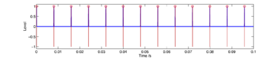
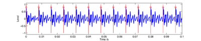
Figure 46 --- A pulse train with a pulse rate of 125Hz (8ms pulse interval) (blue) and the pulse times (red).

Figure 47 --- A synthetic, three-formant, /a/ vowel with a pulse rate of 125Hz (8ms pulse interval) (blue) and the associated pulse times (red).

In the case of the click train and synthetic vowels, it is simple to ensure that the pulse times are known exactly. In the case of the real stimuli, it is possible to generate stimuli with known pulse times by first analysing the signal with STRAIGHT, and then re-synthesising with a known pitch track. Examples of the various synthetic stimuli and associated pulse times are shown in Figure 46 and Figure 47.

An added attraction of these stimuli is that they can easily be added together to create composite stimuli in order to test the effectiveness of strobing systems in multi-source environments, or even to test future systems that segregate stimuli on the basis of the source characteristics.

Methods

Using the synthetic stimuli detailed above, it is possible to test the various strobing systems on some basic criteria. We are interested in how many strobes there are in each channel for each pulse of the input sound, and what proportion of the pulses are correctly strobed upon. This gives a reasonable measure of how the strobe detection system is performing.

To test for the number of strobes per cycle in a single-source sound, a simple sliding window approach can be taken. The NAP and strobes are windowed into sections that are the width of the inter-pulse interval. Each section starts at the known pulse time, and the number of strobes in each section is counted. The system is deemed to be working correctly if there is exactly one strobe in each channel for each windowed section.

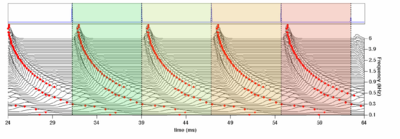
Figure 48 --- Windowing system for assessing the accuracy of strobe detection systems. There should be one strobe point in each channel within each of the four coloured windows if the system is working perfectly.

Figure 48 shows the windowed segments used by the single-source strobe detection system. If there is a one strobe per section in each channel, then the system is deemed to be working perfectly.

For multi-source sounds, this evaluation becomes slightly more complex, as the windows of interest are different for the different sources. In this case, the NAP and strobes are analysed sequentially. The pulse times are arranged in the order in which they occur (regardless of which source they came from). The system then iterates through the sequentially-ordered pulse-times, looking forward from the pulse time in each channel, and assigns the first strobe that it finds within the interval to that pulse. That strobe is then `claimed' by the strobe process, and cannot be used again. Once the complete sound has been processed, the system iterates over the remaining strobe points, and finds those intervals where there are unclaimed strobes. These intervals are marked as containing errors. This tests that the total number of strobes is roughly the same as the total number of pulses, and that the strobes occur at a reasonable rate. However, due to the slightly different methodology between the single-source and multi-source cases, the two sets of results cannot be compared directly.

Results

The following configurations of source stimulus were tested with various strobe algorithms and filterbanks:

Single-rate pulse train
Frequency-swept pulse train
Synthetic vowel
Two pulse trains with different rates
Two synthetic vowels with different rates

For the single-source stimuli, all the available strobe algorithms were tested, including the 'constrained thresholding' and 'event time back-projection' schemes described above. For the two-source cases, the best-performing systems from the single-source tests were tested again. These were the 'local maximum' system and the two newly-developed systems.

Each of the algorithm variants is given a score from 0 to 100% on its ability to get the timing of the strobe points right, and the mean number of strobes per pulse is reported. This value is expected to be around 1 if the system is performing well.

Single-source stimuli

In the first experiment, a 200ms click train with 8ms between clicks was used as the input stimulus to a set of filterbanks and strobing algorithms. Each system was assessed with a percentage score for the proportion of windowed sections with exactly one strobe in each channel, and an overall number of strobes per pulse in each channel. <tablenameRef name="pulse_train_results"/> shows the results from this experiment.

<tablename name="pulse_train_results"/> Pulse train - 200ms length, 8ms repetition rate. Line 1: percentage of pulses correctly identified. Line 2: mean number of strobes per pulse
Algorithm	dcGC	PZFC	log(gammatone)	linear gammatone
peak	13.8%	9.1%	9.9%	10.1%
	6.82	9.92	10.1	9.47
temporal shadow	56.4%	24.1%	9.0%	12.2%
	1.40	1.82	3.65	2.17
local maximum	95.6%	92.9%	89.5%	94.2%
	0.96	0.93	1.02	0.98
constrained threshold	95.9%	93.7%	92.7%	95.6%
	0.97	0.94	1.00	0.97
back-projection	90.3%	84.6%	92.0%	88.9%
	0.92	1.00	0.92	0.92
parabola	87.9%	80.3%	72.9%	86.1%
	1.00	0.96	1.11	1.04
bunt	89.3%	85.8%	59.5%	81.5%
	0.94	0.90	1.01	0.91
lyon	0.0%	0.0%	0.1%	0.1%
	4.23	4.23	4.23	4.23

In the second experiment, the pulse train was swept in pulse interval from 10ms between pulses to 5ms between pulses. The total stimulus duration is 1 second. <tablenameRef name="swept_pulse_train_results"/> shows the results from this experiment.

<tablename name="swept_pulse_train_results"/> Swept pulse train - 1000ms length, 10ms - 5ms repetition rate. Line 1: percentage of pulses correctly identified. Line 2: mean number of strobes per pulse
Algorithm	dcGC	PZFC	log(gammatone)	linear gammatone
peak	14.3%	9.2%	10.4%	10.4%
	6.43	9.14	9.9	9.07
temporal shadow	63.7%	32.6%	11.5%	15.2%
	1.36	1.77	3.62	2.10
local maximum	98.9%	96.8%	94.3%	98.2%
	1.00	0.97	1.05	1.00
constrained threshold	93.4%	92.3%	91.4%	93.1%
	0.94	0.93	0.99	0.95
back-projection	94.9%	95.4%	96.8%	91.7%
	0.99	1.00	1.00	0.99
parabola	91.0%	85.1%	77.8%	85.9%
	0.94	0.95	1.05	0.99
bunt	89.5%	88.0%	60.7%	83.1%
	0.94	0.92	1.01	0.91
lyon	5.5%	5.1%	5.4%	5.5%
	3.99	3.99	3.99	3.99

In the third experiment, a synthetic three-formant /a/ vowel was used. The stimulus duration was 200ms and the pulse interval was fixed at 8ms. <tablenameRef name="synthetic_vowel_results"/> shows the results from this experiment.

<tablename name="synthetic_vowel_results"/> Synthetic vowel - 200ms length, 8ms repetition rate. Line 1: percentage of pulses correctly identified. Line 2: mean number of strobes per pulse
Algorithm	dcGC	PZFC	log(gammatone)	linear gammatone
peak	10.3%	5.1%	10.2%	8.5%
	9.15	9.33	11.56	10.90
temporal shadow	40.9%	19.1%	9.0%	19.1%
	1.82	1.93	4.21	2.38
local maximum	95.2%	82.1%	82.2%	92.9%
	0.97	0.84	1.10	0.99
constrained threshold	95.7%	82.5%	72.5%	94.9%
	0.97	0.84	1.21	0.98
back-projection	87.4%	3.35%	88.3%	88.2%
	0.96	1.73	0.96	0.96
parabola	85.5%	72.7%	66.9%	76.2%
	1.03	0.93	1.18	1.16
bunt	61.5%	75.6%	44.4%	80.1%
	1.24	0.91	1.10	0.94
lyon	0.0%	0.0%	0.1%	0.1%
	4.23	4.23	4.23	4.23

Multi-source stimuli

The test system described above is less robust for the multi-source stimuli than it is for the single-source stimuli. For this reason, only those systems which were seen to perform particularly well with the single-source stimuli are assessed in this section. The three systems assessed are the 'local maximum' criterion and the new 'constrained threshold' and 'back-projection' systems. The results in this section are not directly comparable to the results for single-source stimuli, but these results do allow for basic comparison between algorithms.

The first stimulus is two pulse trains of the same amplitude, one with a repetition rate of 5ms and one with a repetition rate of 8ms. The total duration was 200ms. <tablenameRef name="two_pulse_train_results"/> shows the results from this experiment.

<tablename name="two_pulse_train_results"/> Two click trains - 200ms length, 8ms repetition rate and 5ms repetition rate Line 1: percentage of pulses correctly identified. Line 2: mean number of strobes per pulse
Algorithm	dcGC	PZFC	log(gammatone)	linear gammatone
local maximum	32.9%	30.3%	46.5%	33.7%
	0.33	0.30	0.46	0.34
constrained threshold	43.6%	52.2%	50.8%	43.3%
	0.39	0.54	0.51	0.43
back-projection	56.9%	50.7%	66.7%	57.2%
	0.58	1.06	0.70	0.58

The second stimulus is two synthetic vowels, an /a/ vowel with an 8ms pulse rate and an /i/ vowel with a 5ms pulse rate. The two vowels had the same amplitude. <tablenameRef name="two_vowels_results"/> shows the results.

<tablename name="two_vowels_results"/> Two synthetic vowels - 200ms length, 8ms repetition rate /a/ vowel and 5ms repetition rate /i/ vowel. Line 1: percentage of pulses correctly identified. Line 2: mean number of strobes per pulse
Algorithm	dcGC	PZFC	log(gammatone)	linear gammatone
local maximum	37.9%	33.4%	47.6%	38.8%
	0.38	0.33	0.48	0.39
constrained threshold	44.1%	55.3%	52.8%	44.3%
	0.44	0.69	0.53	0.48
back-projection	62.8%	18.5%	60.4%	64.4%
	0.81	1.46	0.63	0.70

Discussion

The new constrained threshold and back-projection algorithms work well, both for single sources and combined sources. For single sources, the local maximum strobe criterion and the constrained threshold system exhibit very similar performance. This is, in many ways, unsurprising. It shows that the designers of the local maximum system were sensible in their choice of constraints, and used values which were already near optimal.

The performance of the local maximum and constrained threshold are comparable for single sources. For multiple sources, the constrained threshold system performs better (due to the faster decay rates in high-frequency channels) but the improvement is only very slight. The back-projection system works well (except in the case of the PZFC) and is much better than the others in the multi-source case. However, it remains a computationally expensive alternative. For the purposes of large-scale processing of datasets, computational load is a critical concern. As a rough benchmark, the constrained threshold strobe system takes about 10 seconds to process a 2 second noise in AIM-MAT on a 2.4GHz Intel Core 2 Processor. The back-projection system takes around 100 seconds to run on the same stimulus, so there is roughly an order of magnitude performance decrease associated with using back projection.

The back-projection system does not work well with the PZFC filterbank in all cases. As discussed above, it was necessary to increase the strobe threshold decay time for the thresholding system in the PZFC case because the dynamic range of the measured strobe probability was smaller than for the other filterbanks. Despite increasing the decay time, the back-projection system fails on the single-source vowel stimulus because the dynamic range is still too small. Further work to improve the performance of the PZFC with the back-projection strobe algorithm should be directed towards defining a 'canonical' filterbank impulse response from the PZFC, which can be compared with the impulse response in a range of AGC configurations. It is also the case that the zero-crossings of the PZFC shift with level in the current implementation. Replacing the current PZFC with a version where the zero-crossings do not shift with level may help aleviate the strobing problem.

The Lyon strobe detection system with a parabolic window performs very badly with respect to the criteria for a good strobe mechanism. The strobes-per-pulse values are identical for all filterbanks since the system has to produce a fixed number of strobes for a given stimulus length, and so performance can never be optimal. However, when this system was incorporated into the sound-effects recognition system described in chapter 6, it was found that performance with a SAI based on this system is actually slightly better than performance with a SAI which uses strobes from a simple thresholding based system. In this case, at least, is seems that optimal strobe detection is not such an important requirement.

Conclusions

Performance with the new strobe finding mechanisms based either on 'constrained thresholding' or 'event time back-projection' shows some slight improvements over previous systems. However, the change is not that great, and the 'local maximum' variant of the 'temporal shadow' strobe criterion performs almost as well as the new mechanisms in many cases. The default parameters for the temporal shadow criterion do not vary as a function of channel centre frequency, but they are similar to the parameters determined by the constraints described above for mid-range centre frequencies; the 5ms default strobe lag of the 'local maximum' system corresponds to the rise time of a driven filter at around 1600Hz, or an undriven filter at around 600Hz. The designers of previous strobe detection systems were careful to choose parameters which gave the best results possible, and succeeded in correctly identifying a good set of parameters for the dynamics of the filterbank they were using.

In this analysis, I have placed assumptions implicit in previous strobe detection systems on a firmer theoretical basis, and confirmed that the choice of constants made for these systems was reasonable. While the improvement gained by the 'constrained threshold' system described here over previous systems is small, the understanding of filterbank dynamics should prove useful for the development of future strobe detection systems.

An alternative strobe detection system was also introduced that compares the NAP to the impulse response of the filterbank at every time step. While this system is extremely effective at 'back-projecting' to find the original strobe time, it is inefficient and so cannot be used in a large-scale machine hearing system at this point in time. Further work would also be required to tune the parameters of this system in order to make it work correctly with the PZFC filterbank.

In the next chapter, the features developed in chapter 2 are computed from the stabilized auditory image, rather than from the cochleogram. We hypothesise that the stabilized features produced with strobed temporal integration will be more noise-robust than those generated from the NAP. The syllable recognition system developed in chapter 2 provides an excellent test-bed for the alternative features.

Features from the Auditory Image

In chapter 2 of this thesis, I took an observed property of the human auditory system -- that it is capable of correctly recognising pulse-resonance sounds which have had their resonance scale modified to well beyond the normal range of experience -- as the inspiration for a scale-shift invariant feature representation. The features were tested using a database of syllables which had been scaled to simulate speakers with a range of vocal tract lengths and glottal pulse rates. In chapter 3, I focused on the properties of strobed temporal integration, a mechanism whereby the auditory system might generate a stabilized representation of the neural patterns coming from the cochlea. In this chapter the feature representation developed in chapter 2 and the stabilised auditory images generated by strobed temporal integration are combined to create a feature representation which we hypothesise should have the scale-invariance properties of the original features and the noise-robustness properties of the stabilised auditory image. The various feature variants are compared with each other and with the standard MFCC features used in chapter 2.

The stabilised auditory image

The auditory image model (AIM) (Patterson et al., 1995) provides a framework for creating a stabilized auditory image (SAI) from the output of a filterbank. This representation of the signal is stable for sounds which are perceived by listeners as being stable. Theoretically, it is also more noise-robust than a simple filterbank representation (Patterson et al., 1992; Patterson, 1994b), since the strobed temporal integration process causes the neural patterns associated with successive cycles of a periodic sound to reinforce each other in the SAI.

The stabilised auditory image (SAI) is a two-dimensional representation of an input sound. A single SAI is a snapshot of the audio in a short window around a point in time. The SAI changes continuously with time, and successive snapshots can be concatenated to make a movie of these two-dimensional frames. The first dimension of an SAI frame is simply the spectral dimension added by the filterbank. The second dimension comes from the strobed temporal integration process by which an SAI is generated. Strobed temporal integration works by locating prominent peaks, or 'strobes', in the incoming signal and calculating 'lags' relative to these times. These peaks are most commonly associated with the pulses in pulse-resonance sounds, for example the glottal pulses in speech. When a strobe occurs in a channel, a short segment of the signal following the peak in that channel is added to a buffer, starting at zero lag. The signals following multiple strobe points add constructively in the buffer. This process leads to a stable spectro-temporal representation of the microstructure in the signal following each pulse in the input sound.

The SAI was introduced in chapter 1, and the process by which strobe points can be detected was discussed at length in chapter 3. In this chapter, features generated from SAI-based representations are developed and tested. A useful property of the SAI is that it is stable when the input sound is perceived as being stable. Temporal averaging is performed in a 'smart' way - such that there is no 'beating' between the windowing function and the pulse rate of the incoming signal (Kawahara and Irino, 2004). The strobed temporal integration process also makes the representation of pulse-resonance sounds robust to interfering noise; pulse-resonance sounds will tend to be accentuated in this representation, since the strobed temporal integration process will lead to multiple pulses and resonances being placed on top of one another in the SAI, causing them to interfere constructively. By contrast, noises which have no temporal regularity will not be reinforced in this way, and will appear at a lower level relative to the pulse-resonance sounds since they will not, in general, interfere constructively.

In this section, the noise-robustness of the SAI is tested, using the syllable-recognition task described in chapter 2. Instead of generating features from the NAP, AIM-C was used to generate a SAI, which was then transformed into a size-shape image (SSI). To generate features for use in a recognition system, various spectral profiles of this image are computed and used as the input for the Gaussian fitting scheme described in chapter 2.

SAI marginals

Figure 49 -- An SAI with its temporal and spectral profiles

To a first approximation, it is possible to summarise the SAI by its marginals -- that is the vectors describing the mean of the SAI along its horizontal and vertical dimensions. These marginals are known as the `temporal profile' and `spectral profile' of the image. The SAI spectral profile is essentially a smoothed and temporally averaged version of the filterbank output. The temporal profile summarises information concerning the time intervals between prominent NAP pulses, and the time intervals in the fine structure following prominent pulses. Figure 49 shows an SAI, together with its temporal and spectral profiles.

Undersampling

Having said that the SAI segregates the pulse rate information and the resonances, it is still the case that changes in the pulse rate must have an effect on the structure of the resonances in the signal. This effect is easy to see by considering a pulse-resonance signal in the frequency domain. In this domain, a single damped resonance corresponds to some continuous frequency distribution. An idealised pulse train will have a frequency spectrum that also looks like a pulse train, with all harmonics of the pulse rate present in the spectrum. The pulse-resonance generation model has a stream of pulses exciting resonances of the vocal tract or other body. The time-domain pulse train and resonance are convolved to give the pulse resonance signal. This corresponds to a multiplication of the resonance envelope by a comb of peaks in the frequency domain: the resonance is `sampled' at the harmonics of the driving function. Thus although the pulse-resonance production mechanism allows a signal to be generated over longer time scales than the length of a single damped resonance, in doing so it causes information about the structure of the resonance to be lost. At higher pulse rates, the spectrum is sampled more sparsely, and so more information is lost. This `undersampling problem' is described in detail by de Cheveigné and Kawahara (1999).

The SSI

The 'scale-shift covariant' or 'size-shape' image (SSI) is another two-dimensional frame-based representation of the audio signal. It is obtained from a transformation of the SAI, and is a VTL covariant representation of the input signal. This means that changes in VTL correspond to simple shifts of the image. Patterson et al. (2007) provide an overview of the mathematics of the SSI and the process of generating images.

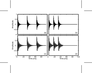
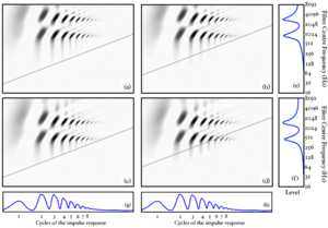
Figure 50 --- Four synthetic two-formant vowels, that differ in pitch and VTL. The upper two vowels (a) and (b) are for a short VTL with low and high GPR respectively. The lower two vowels (c) and (d) are for the same two GPRs with a longer VTL. This figure was prepared by Ralph van Dinther in connection with Patterson et al. (2007). Used with permission.

Figure 51 --- Idealised SSIs for one cycle of four synthetic two-formant vowels, as shown in Figure 50. This figure was redrawn from a figure by Ralph van Dinther. Used with permission.

The SSI is calculated from the SAI by taking the signal in each channel, and truncating it to leave the portion between zero-lag and the first peak associated with the next excitation pulse, that is the peak that completes the pitch period. This peak can be found in most cases by looking for the next highest peak in the SAI channel after the peak at zero-lag. Each of these truncated signals is then plotted as a function of cycles of the impulse response for the filter in that particular channel. In practice, this means that the time axis of each channel in the SAI is independently dilated by an amount proportional to the centre frequency of the filter in that channel. This has the effect of lining up the cycles of the impulse response of the filters. Interestingly, this transformation also has the effect of normalising out the faster decay rate of higher-frequency resonances in pulse-resonance sounds. This means that for a simple VTL change, because the auditory filterbank introduces a quasi-logarithmic scale on the vertical axis of the SSI, the pattern of formants in the SSI will shift as a unit up and down the vertical (cochlear place) axis of the image. With a logarithmic horizontal 'cycles' axis as well, the truncation of the signal at the pitch period of the incoming waveform has the effect of placing a diagonal `cutoff line' in the SSI at the point where the next pitch period begins. As pitch changes, this cutoff line retains the same gradient, but shifts its position up and down the image.

Figure 51 shows idealised SSIs for the four vowels in Figure 50. The SSIs are `idealised' in the sense that they are generated from a single cycle of the source vowel. The blue diagonal line in each case shows the cutoff line where the next pitch period would begin. In panel (d) where the source vowel has a high pitch and is from a long vocal tract, the pitch cutoff line clearly interferes strongly with the formant pattern. This is another manifestation of the undersampling problem.

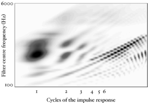
Figure 52 --- SSI for a real human /a/ vowel.

Figure 52 shows an SSI for a real human /a/ vowel. The pitch cutoff line is clearly visible as a strong diagonal in the image. Beyond this line, subsequent cycles of the waveform are squashed into a smaller and smaller space. The useful information in such an image is all in the area to the left and above the pitch cutoff line.

If it is possible to do accurate pitch detection in the SAI, then the SSI can be truncated at the pitch-cutoff line as it is generated. Accurate pitch detection is straightforward for single-source problems, however for images that contain multiple independent sources, the problem becomes more challenging.

The form of the information in the SSI

Figure 53 --- The form of the information in the SSI.

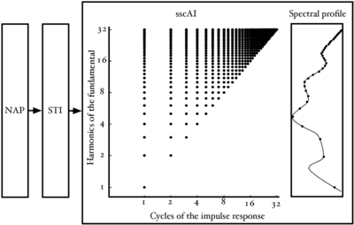
Figure 53 shows the points in the SSI where the information in pulse-resonance sounds is concentrated. Channel centre frequency is along the vertical dimension and time interval along the horizontal dimension. The units in the vertical dimension are harmonics of the fundamental. The units in the horizontal dimension are cycles of the impulse response.

In the frequency dimension, the points of interest are dictated by the pulse rate of the waveform. We have seen previously that for a pulse-resonance sound with a nonzero pulse rate, the spectral envelope will be sampled at the harmonics of the pulse rate. These harmonics are logarithmically spaced on the ERB axis of the auditory filterbank. This leads to the logarithmic spacing of points in the frequency dimension. In the time-interval dimension, the main points of interest are the peaks of the cycles of the impulse response in each channel. The response of the filter can be approximated by the amplitudes of the time domain peaks.

Dimensionality reduction

The transforms that convert a sound into an auditory image are intended to project the incoming signal into a space where pulse-resonance sounds are enhanced relative to background noise, and changes in acoustic scale leave the pattern of information largely unchanged, save for a spatial shift. While noise robustness and scale invariance are attractive properties, the transforms used to construct the space produce an explosion in the data rate which is a serious problem for an engineer trying to develop a speech recognizer. Whereas the data rate of the original sound is on the order of 300kbps, the data rate of the auditory image is on the order of 30Mbps. There are clearly substantial redundancies in the SAI and it behoves us to try and find a compact vector of features that summarises the signal and reduces the data-rate burden, if the SAI is to be used as the basis of a recognition system.

Chapter 6 details a method of producing a compact summary of features from the output of AIM-like models, and compares them to MFCCs, the traditional features in automatic speech recognition and sound classification. In the remainder of this chapter, the Gaussian features developed in chapter 2 are used to summarise spectral slices of the SSI, and the robustness of these features to noise is compared with that of the MFCCs and the features derived from the NAP in chapter 2.

Profiles and slices of the size-shape image

The SSI can be generated either with or without the pitch cut-off line. In the case of an SSI without the pitch cutoff, the second and subsequent pitch periods are `squashed' together in the lower right corner of the image. To generate the pitch cutoff for the experimental features described below, the temporal profile of the SAI was taken and the largest peak after the zero-lag peak is taken as the most prominent pitch period in the signal. There is a short `lockout' period of 4.6ms after the zero-lag peak, during which peak detection is suppressed, to allow the temporal profile to decay sufficiently. This allows detection of pitches up to around 217Hz. This allows for coverage of all pitches in the syllable database used for training and testing. However, more generally, spoken pitches may exceed this value and so the system would need to be modified to include a more robust pitch tracker in order to use the truncated SSI for features.

For both the full SSI and the truncated SSI, features were generated in two different ways. In each case, a spectral profile was constructed from the SSI and this was used with the Gaussian fitting procedure introduced in chapter 2. In the first variant, the spectral profile of the complete SSI was taken and used for fitting. In the second variant, a vertical `slice' of the SSI around the peak of the first cycle of the impulse response was taken, and the spectral profile of just this slice was taken.

In the case of the pitch-truncated SSI, for higher pitches, the lower-frequency regions of both these profiles may be zeroed-out. This can lead to a discontinuity in the spectral profile at that point. No attempt was made to smooth out this discontinuity before passing the profile to the Gaussian fitting procedure.

Figure 54 shows the regions of the SSI used to calculate the four feature variants used in the experiments, and the spectral profile for each region.

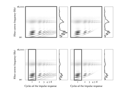
Figure 54 --- The four SSI variants used in the experiments. Each SSI is for the same /i/ vowel, spoken by a male. The left-hand SSIs are without the pitch cutoff, the right-hand SSIs are with the pitch cutoff. The grey boxes denote the region which is included in the spectral profile calculation. Spectral profiles for the region in the grey box are plotted to the right of each SSI. The large boxes cover the whole image, the small boxes just cover the first cycle of the filter impulse response in each channel.

Experiments

Comparison with features from the NAP

Recognition performance with these new SSI-based features was compared with that of the NAP-based features of chapter 2, using the syllable recognition task of chapter 2. The NAP features were compared with each of the four feature variants derived from the SSI. In these initial experiments, there was no noise background.

For each of the variants, the spectral profiles of successive image frames were fitted using the Gaussian fitting procedure described in chapter 2. This generates a 4-dimensional feature vector, containing the three relative weights of the Gaussians and a total energy term, as before. Delta, and delta-delta coefficients were calculated from these features, and the complete 12-dimensional feature vector was passed to the HMM recognition system described in chapter 2.

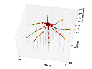
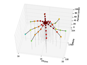
Figure 55 --- Scaled syllable recognition performance on the full SSI profile with no pitch cutoff.

Figure 56 --- Scaled syllable recognition performance on the full SSI profile with the pitch cutoff.

Figure 55 shows the performance of the whole-SSI features with no pitch cutoff on the syllable database. Performance is 84.8% overall, falling to a low of 31.6% at the shortest VTL. Figure 56 shows the performance for the SSI features with the pitch cutoff. Performance in this case is somewhat improved, rising to 86.7% overall, and 37.8% at the shortest VTL. The improvement in performance is mainly due to the stability of the results across the pitch dimension when there is a pitch cutoff on the SSI.

Overall performance on the NAP-based features was 93.8%, falling to a low of 71.9% for the speaker with the shortest vocal tract. The data are replotted from chapter 2 in Figure 57 for comparison. So, in clean speech, overall performance with NAP-based features is somewhat better than for SSI-based features derived from the whole SSI.

Figure 57 --- Scaled syllable recognition performance on the original NAP-based features.

Figure 58 and Figure 59 show the results (with and without the pitch cutoff, respectively) for the features generated from the cycle-1 slice of the SSI. Overall performance with no pitch cutoff is 79.0%, and 81.3% with the pitch cutoff. In the no pitch cutoff case, performance is again lowest for the speaker with the shortest vocal tract, falling to 27.0%. For the pitch cutoff case, performance is lowest on the speaker with the longest vocal tract at 27.6%.

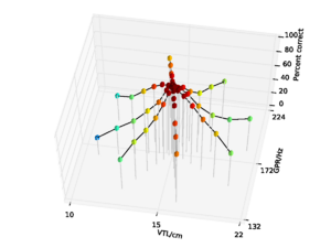
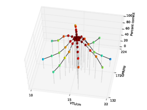
Figure 58 --- Scaled syllable recognition performance on the SSI cycle-1 profile with no pitch cutoff.

Figure 59 --- Scaled syllable recognition performance on the SSI cycle-1 profile with the pitch cutoff.

In general, then, when there is no background noise, performance with the SSI-based features is lower than for the NAP-based features, and the SSI-based features are more susceptible to changes both in pitch and in VTL. This is a somewhat surprising result, since to a large extent, the energy distribution in the SSI profile is the same as that in the NAP. Performance is still better than with the MFCCs without VTLN, however, where overall performance was 75.5%. Performance with the SSI features does not approach that of MFCCs with optimal VTLN at 99.2%.

Testing in noise

So far, the recognition experiments in this thesis have all been performed on clean audio data. However, how a system performs in noise is also an important consideration for practical speech recognition. As discussed above, the SSI is expected to provide a representation of the input signal which is more robust to interfering noise than a purely spectral representation like the smoothed NAP profile or the mel-frequency spectrum. This hypothesis was tested by training and testing the syllable recognition system in noise. The recogniser was trained on features generated from syllables presented in a background of noise at a range of levels, and then testing performance of the same recognition system on each noise level in turn, and recognition performance on the features was measured as a function of signal-to-noise ratio (SNR).

To create the noisy data set, the syllables in the database were mixed with pink (1 / f) noise using the `sox' sound processing tool. The normalised RMS level of the voiced portion of the syllable was used as the reference level to establish SNR. Stimuli were generated with SNRs from +42 dB down to 0 dB, in 6 dB increments. SSIs were generated from the input sounds using AIM-C, and MFCCs were generated using HTK, as before. The four different types of SSI features (whole SSI profiles and cycle-1 slices, with and without the pitch cutoff) were computed for all SNRs. MFCC features, with and without optimal VTLN, were also computed for all SNRs. HMMs were trained on the nine inner speakers from the spoke pattern, as before. However, in this case each training example was presented with an SNR picked randomly and uniformly from the complete range of SNRs. Testing was performed with all examples from the same SNR. As in chapter 2, a range of HMM configurations were tested. As before, the pattern of performance was found to be similar across a wide range of HMM configurations, and the results are presented on a representative point in the feature space where performance was found to be near optimal for all the feature types, in this case a 2-emitting-state HMM with 4 output components after 8 training iterations of the HMM.

Figure 60 shows overall recognition performance as a function of SNR for MFCC features, with and without optimal VTLN, and for the features from the AIM NAP. As in the case of clean speech, performance is low on the standard MFCCs due to their lack of scale-shift invariance, and is high for MFCCs with VTLN. For the features from the AIM NAP, performance is consistently slightly lower than for the features with VTLN, and the two curves follow the same trajectory as noise level increases.

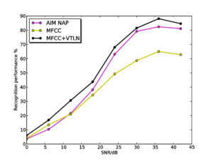
Figure 60 --- Recognition results for the AIM NAP profile and MFCC features, where the model was trained and tested in noise.

Figure 61 and Figure 62 show the results for the whole-SSI profile and SSI cycle-1 slice features respectively. In each plot, results are shown both with and without the pitch cutoff. In each case, the results vary very little depending on whether the pitch cutoff is used or not. In each case, there is a very slight benefit to using the pitch cutoff at high SNRs, but the cutoff is detrimental at low SNRs. This change is likely to be due to the simple algorithm used to compute the cutoff line, which just finds the highest peak in the temporal profile of the SAI, and takes this to be the most salient pitch in the input signal, making a hard decision on the input pitch. Once noise is added, this process will become less robust, and less consistent across different utterances so as the noise level increases the process starts to do more harm than good. A potential way of countering this effect would be to make a 'softer' pitch decision; this could take the form of a simple roll-off function that is applied to the edge of the SSI (for example a tanh window). The width of the roll-off could be modified depending on the pitch strength of the dominant signal pitch.

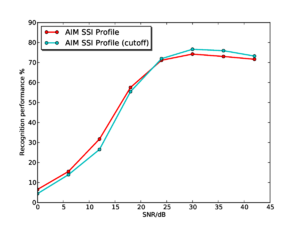
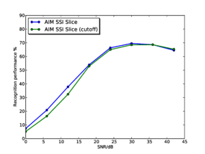
Figure 61 --- Recognition results for the whole-SSI profile AIM features, where the model was trained and tested in noise.

Figure 62 --- Recognition results for the SSI-slice profile AIM features, where the model was trained and tested in noise.

Figure 63 shows the results for the AIM SSI features (without pitch cutoff) and the AIM NAP features for comparison. Performance with the SSI-based features starts from a lower baseline, as as seen in the experiments on clean syllables. However, interestingly, performance degrades far less rapidly as the noise level increases for the SSI-based features, such that by 24dB SNR, the SSI-based features are outperforming the NAP-based features. Performance with the SSI-based features remains consistently higher right down the 0dB SNR. Furthermore, at SNRs of 12dB and below, the SSI slice-based features have the best performance, despite having started off with the lowest recognition rates in clean speech.

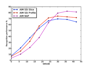
Figure 63 --- Recognition results for variants of the AIM features, where the model was trained and tested in noise.

Conclusions

The results with the SSI-based features suggest that there is indeed a benefit to using a representation of audio based upon the stabilised auditory image to improve noise-robustness in audio analysis tasks - however, baseline performance of the SSI-based systems is lower for clean input than that with simpler spectral-based representations. These results clearly point the direction for further research into the use of auditory models for content-based audio analysis tasks. The next step will be to explore whether it is possible to improve recognition performance on the SSI to bring it in line with that on the NAP alone. Initial inspection of the SSI profiles suggests that there is increased variability in these profiles relative to the smoothed NAP profile. This increased variability appears to be due in part to a feature of the strobed temporal integration process chosen to generate the images. In the version of strobed temporal integration used, SAIs are generated taking into account all strobe points which occurred before the snapshot of the auditory image is taken. This can lead to cases in which an SAI is generated when a strobe has recently occurred and only some data is available about what follows that strobe. If there is not enough signal available in a given channel to fill the complete width of the SSI, then the signal will be added up to the point where the signal stops, which can lead to small discontinuities in the generated image.

In the experiments in this chapter and in chapter 2, two important properties of auditory models have been demonstrated. First a macroscopic observed property of the auditory system, that it appears to perform automatic scale-normalisation, was used to inform the development of scale-shift invariance of the features. Secondly, a predicted property of the image stabilization process, that it creates auditory images which are more robust to interfering noise, was tested with the scale-shift invariant auditory features. However, these two properties of the auditory features are independent of one another, and it should be possible to demonstrate these two effects independently. One possible way to do this would be to summarise the spectral profile of the NAP and SSI by a more MFCC-like representation that does not have the scale-shift invariance properties of the Gaussian fitting procedure used in the above experiments. This could be done by taking a DCT over the logarithmically-compressed spectral profile of the NAP or SSI. Given the results presented above, the features generated from the SSI would be expected to be more noise-robust that those generated from the NAP.

Further work

In this chapter I have tested one possible feature representation generated from the SAI in a constrained task. However, there are many opportunities for creating a richer feature representation from the stabilised auditory image representation. Given the effectiveness of the DCT in lowering the dimensionality of the spectrum in MFCCs, a potential feature of interest might be created by taking the first DCT coefficient from each column of the SSI - generating a per-cycle MFCC-like representation. To include scale-shift invariance, the DCT could be replaced with a Fourier transform, and the phase discarded. Such features would correspond to a subset of the Mellin image (Irino and Patterson, 2002). These more general features could be assessed by trying them in a range of tasks where MFCCs are normally used.

Looking at the wider problem of how to process SAI-based representations into usable features, the major concern is how to perform dimensionality reduction in a manner which retains as much of the interesting information that it contains as possible while producing a feature vector which is sufficiently compact to be useful.

In chapter 6, one such system is developed: each SAI frame is decomposed into a set of blocks of different scales, and the contents of each block is converted into a sparse vector by use of a 'codebook' of common patterns seen in that block. This multi-scale approach to the problem of feature extraction is a crude but effective way of analysing different parts of the SAI in an independent manner, and removes the dependence of the current systems on the expensive fitting of spectral profiles with a constrained GMM. The feature representation developed in chapter 6 is considerably richer than these simple GMM-based features and allows for its use on a more open-ended task.

Compressive Auditory Filtering

So far, this thesis has studied the properties of the human auditory system in gradually increasing levels of detail. At the largest scale, the feature representation developed in chapter 2 aimed to emulate the observed behaviour of the system as a scale-invariant preprocessor, which can provide a representation of pulse-resonance communication sounds independent of the pulse rate and the resonance scale of the sound.

'Zooming in' to look at another level of detail, in chapter 3 the process of strobed temporal integration was investigated and placed on firmer theoretical ground. In doing this, it was hypothesised that the auditory images generated using strobed temporal integration should be more robust to noise than features generated from more simple, purely spectral models. This hypothesis was investigated in chapter 4 by adapting the auditory features developed in chapter 2.

Having modelled and observed the large-scale behaviour of the auditory system, and then developed a particular model of the post-cochlear neural processing, this chapter 'zooms in' again to look in finer detail at the behaviour of the cochlea, and in particular its response at very short timescales. The cochlea is perhaps one of the more well-understood components of the auditory system, and there is a wealth of data on the spectral shape of the human auditory filter, and the fine-timing properties of the mammalian cochlea.

The dynamic range of audio signals is orders of magnitude larger than the dynamic range available to encode those signals in the auditory nerve. This means that the auditory system has to perform some sort of compression on the incoming signal in order to represent it effectively with a neural code. It is perhaps surprising to find that the auditory system performs this compression within the auditory filter itself; it uses mechanical feedback from the outer hair cells (OHCs) to dynamically modify the motion of the basilar membrane, and so the signal encoded by the inner hair cells. One important advantage of this approach is that it makes it possible to perform the dynamic range compression with an extremely fast time-constant. The auditory filter is able to compress the peaks of the waveform within a single cycle, and leave the zero-crossings effectively unchanged.

Models of auditory filtering attempt to describe mathematically the processing performed by the cochlea on an incoming sound, which ultimately leads to a neural response. They are a mathematical abstraction of the response of the complex physiological systems in the cochlea to stimulation by an incoming pressure wave. There exist a number of excellent descriptions of various parts of the history of these models, for example Lyon (1996) and Patterson et al. (2003). The introduction to this chapter briefly covers the major points of the various models, and introduces a set of increasingly more complex criteria that an auditory model must fulfil in order to accurately model the human auditory system.

An important feature of the more recent models of the auditory filter is their ability to deal with dynamic compression performed by the cochlea. In this chapter, two recent models of the auditory filter that perform dynamic compression are discussed and analysed. The models are the dynamic, compressive gammachirp (dcGC) (Irino and Patterson, 2006; Irino, Walters and Patterson, 2007) and the pole-zero filter cascade (PZFC) (Lyon et al., 2010). The two filter models are compared in their response to a number of test stimuli to assess the response of the dynamic, time-varying compression that they both implement.

The studies presented in this chapter provide some evidence that dynamic, within-cycle, compression is a feature of auditory processing which is important for correctly modelling human perception of certain stimuli. The stimuli used in this chapter are iterated rippled noise (IRN) and high-pass filtered harmonic complexes in which the fundamental and lower harmonics of the stimulus are not present. These stimuli illustrate well the ability of the auditory system to process temporal regularity in a signal despite the lack of a strong fundamental harmonic, and thus provide a good test for temporal models of audition.

This chapter does not directly address the problem of whether compressive filtering is a crucial element for a good machine-hearing system, but rather looks at the application of compressive filtering to a particular class of stimuli, the correct representation of which is required in a system which accurately models human auditory perception. This is an incremental step towards understanding exactly which aspects of human auditory processing are necessary for effective machine hearing.

A short history of models of auditory filtering

The presence of a set of simple damped resonances, or filters, in the cochlea was conjectured by von Helmholtz (1875), but the idea of resonances in the human auditory system had been discussed as early as 1605 (Wever, 1949). Fletcher (1940) suggested that the peripheral auditory system could be modelled as a bank of bandpass filters with overlapping passbands, on the basis of his measurements of the threshold for detection of a sinusoid when masked by a bandpass noise with a controlled bandwidth. Descriptions of the response of the auditory filter in the frequency domain, based on the results of tone-in-noise masking experiments, came to be known as the `power-spectrum model of masking' Moore (1995). Power spectrum models deal only with stimuli that are static in time, and which only describe the shape of the magnitude spectrum of the auditory filter in the frequency domain; however, this is enough to quantify the overall shape of the filter's transfer function.

The cochlea is known to have a degree of nonlinearity. The fact that the bandwidth of auditory filters exhibits level-dependence, and the presence of distortion products (Kim et al., 1980), particularly in otoacoustic emissions (Moore, 2003), suggests that there is some sort of 'instantaneous nonlinearity' in addition to an overall compression function (Lyon et al., 2010). Another effect that a cochlear model should be able to account for is two-tone suppression (Moore, 2003; Sachs and Kiang, 1968), where an off-frequency stimulus can cause suppression of the on-frequency response of an auditory neuron. Although the effect was first measured in neurons, there is strong evidence to suggest that it occurs in the cochlea (Rhode and Robles, 1974; Rhode and Cooper, 1993; Ruggero et al., 1992).

A set of desirable properties of a practical auditory filter are set out by Lyon et al. (2010). The list is as follows:

Simplicity of description. Either in the time domain, the frequency domain or in the Laplace domain.
Bandwidth control. Filter bandwidth varies as a function of cochlear place, and of sound level.
Realistic and controllable relationship between peak shape and skirts. After bandwidth, the shape of the filter near the edges of its band is the next most important feature, and this should vary with level.
Filter shape asymmetry.
Gain variation. Gain, as well as bandwidth, varies as a function of level.
Stable low-frequency tail. In order to provide a good match to physiological data, the gain of the low-frequency tail of the filter should not vary much as a function of input level.
Ease of implementation as digital filters. In order to make a good digital filter, the model either needs to be described in terms of poles and zeros, be convertible to such a description, or be approximated by such a description.
Connection to the underlying assumptions about the travelling-wave hydrodynamics of the cochlea.
Good impulse-response timing and phase characteristics: for comparison with physiological measurements, across a range of levels, details such as zero-crossing times can be diagnostic of whether the model is faithful to the mechanics.
Dynamic. In addition to being parameterised by level, the filter should be dynamically variable with a fast time constant, such that the filter can compress the glottal pulses in a pulse-resonance sound.

The auditory models set out below attempt to characterise temporal and spectral characteristics of the auditory filter with varying degrees of fidelity, in order to explain the psychophysical data available on masking, compression and two-tone suppression, and electrophysiological data available on the temporal characteristics of auditory filters.

Roex filters for frequency-domain fits

Early efforts to quantify the shape of the auditory filter in the frequency domain employed the `roex' ('rounded exponential') function to describe data from notched-noise masking experiments in humans (Patterson et al., 1982). While the magnitude of the basic roex has a simple description in the frequency domain (a pair of back-to-back exponentials with a rounded top), the phase response is not defined. This in turn leaves the impulse response undefined and so the roex, like other simple descriptions of the frequency spectrum of an auditory filter, cannot be used to make a time-domain filterbank (Patterson et al., 2003). The initial versions of the roex filter, the $roex(p)$ and $roex(p, r)$ were symmetrical in their frequency response, with the latter adding a second parameter to control the shape of the skirts of the filter. The $roex(p u, p l, r)$ added independent control of the parameters for the upper and lower sides of the filter in order to take into account the known asymmetry in filter shape, and the $roex(p, w, t)$ also added asymmetry. Various more complicated versions of the filter emerged, with up to six free parameters. In this way, the roex family could be used to fit human masking data very accurately, but at the expense of adding many additional free parameters.

The gammatone family

In the time domain, the gammatone function had been used for many years to model various forms of auditory response. The gammatone is defined in terms of a gamma-distribution ( $A t n - 1 exp( - b t)$ ) multiplied by a sinusoidal tone ( $cos(ω r t + ψ)$ ), and was first used as a model of basilar membrane displacement by Flanagan and Guttman (1960). The function was reintroduced by Johannesma (1972), who used it to characterise the response of the cochlear nucleus, and by de Boer (1975) to describe the cochlear impulse response measured in cats. The term 'gammatone' was first used to describe the function in 1980 by Aertsen and Johannesma (1980). Schofield (1985) demonstrated that the magnitude response of the gammatone could be used to explain human masking data, and Patterson et al. (1988) then highlighted the similarities between the gammatone magnitude response and the shape of the roex function. Thus the gammatone came to be accepted as a model of the human auditory filter, in both the time domain and the frequency domain.

Since the gammatone had a well-defined impulse response, producing systems to model auditory filters was now possible. Martin Cooke produced an early gammatone filterbank while working with Schofield at the National Physical Laboratory (Cooke, 1993), and John Holdsworth produced the Cambridge gammatone filterbank code while working with Roy Patterson. Practical implementations of the gammatone filter exist both as IIR and FIR filterbanks, and many people use the IIR implementation of Slaney which has the attraction of an accompanying Mathematica workbook (Slaney, 1993f). Holdsworth's filterbank code was used successfully over many years as the filterbank in AIM (Patterson et al., 1995).

In its simplest form, however, the gammatone filter is linear, and has a near-symmetrical frequency response around its centre frequency. These properties mean that alone it cannot simulate either the compressive behaviour exhibited by the cochlea, or the asymmetry seen in the auditory filter at high input levels.

Figure 64 – Impulse responses of a gammatone filter (solid line) and a gammachirp filter (dotted line). The chirp parameter,

c

, is

0

for the gammatone and

- 2.0

for the gammachirp

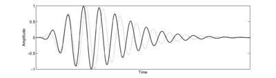
To extend the gammatone, Irino and Patterson (1997) derived the gammachirp filter as the minimum-uncertainty operator for a joint time-scale representation of signals (Cohen, 1993). The derivation is analogous to that of the Gabor function as the minimum-uncertainty operator for a joint time-frequency representation. This is a very deep result, and reinforces the underlying importance of scale in the auditory system. In practice, the gammachirp extends the gammatone by adding a parameter, c, which controls the addition of a log-time term to the carrier ( $cos(ω r t + ψ + c log(t))$ ). This has the effect of making the filter 'chirp' in frequency as a function of time, and adds an asymmetry to the frequency response of the filter. Figure 64 shows the impulse responses of the gammatone and gammachirp filters. The compressive gammachirp (cGC) was first used to fit the simultaneous masking data of Rosen and Baker (1994) and subsets of the masking data from Lutfi and Patterson (1984) and Moore et al. (1990), with the parameter $c$ being allowed to vary as a function of level. They found that it was possible to achieve a similar fit to the masking data with a 4-parameter cGC model as could be achieved with a 6-parameter roex model. Furthermore, the cGC has a well-defined impulse response that can be used to construct a time-domain auditory filterbank.

In practical terms, the cGC can be implemented as a gammachirp filter with an arbitrary value of the chirp parameter, $c$ , cascaded with an `asymmetry function', which is either high-pass or low-pass, depending on $c$ (Patterson et al., 2003). This means in practice that the passive gammachirp filter can be reduced to a static gammatone filter (a gammachirp with $c = 0$ ) and a lowpass asymmetry function. The addition of a complementary high-pass asymmetry function in which centre frequency varies as a function of level allows for a practical cGC filter. Furthermore, the asymmetry functions can be implemented as IIR filters, allowing for an efficient implementation of the filterbank (Unoki et al., 2001).

The dynamic compressive gammachirp filterbank (dcGC) of Irino and Patterson (2006) is a direct descendant of the cGC filter, which models the compressive nonlinearities in the human auditory system. The dcGC is based on the compressive gammachirp (cGC) filterbank Patterson et al. (2003). The dcGC filterbank includes a system for dynamic modification of the cGC filterbank compression parameters in response to the input audio.

Simple representations of the gammatone family in the Laplace domain

Lyon (1997) noted that the representation of the gammatone filter could be simplified by discarding the zeros from the S-plane transfer function to yield an 'all-pole' gammatone filter (APGF). The APGF has fewer parameters than the equivalent gammatone, and has a more controlled behaviour in the tail of the filter. Allowing one zero back into the APGF transfer function yields the one-zero gammatone filter (OZGF); the zero is constrained to lie along the real axis. The special case where the OZGF has its zero at the origin in the S-plane is known as the differentiated all-pole gammatone filter (DAPGF). This extra zero allows more control over the tail of the function than is possible with the standard gammatone function. Furthermore, it provides a simpler way to model the level-dependent gain, bandwidth, asymmetry and centre-frequency shift exhibited by human auditory filters.

Filter cascade models

When considering the analogy between the cochlea and auditory filterbanks, it is important to remember that the cochlea is in fact a complex hydrodynamic system, in which a wave travels along a continuous medium from base to apex. The mechanical properties of the basilar membrane (BM) vary from the basal end to the apical end, and the response of the BM to different frequencies along its length is largely determined by this change (von Békésy, 1960; Moore, 2003). Transmission-line, and more recently, filter cascade models of the cochlea attempt to capture this continuous structure, and describe it as a cascaded sequence of filters. Zweig et al. (1976) used the WKB approximation<ref>The Wentzel–Kramers–Brillouin (WKB) approximation is a technique for approximating the solution of a wave equation, which was originally developed in quantum mechanics. For a wave equation $W (x, t) = A exp(i (k x - ω t))$ , the WKB approximation states that 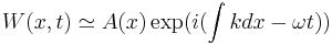$W(x,t)\simeq A(x)\exp(i(\int k dx-\omega t))$ . When k is independent of x, the solution is exact, and as long as k varies only slowly with x, the approximation remains valid. This is equivalent to modelling the slowly-varying properties of the cochlea as a series of discrete filters. See Lyon and Mead (1988) for a complete treatment of the mathematics.</ref> to show that small segments of the cochlea can be seen to act as local filters on the waves propagating down its length, and so it is possible to describe the continuous cochlea as a set of cascaded filters. This led the way for a set of cochlear models known as 'cascade filterbanks' (Lyon, 1998) in which the continuous BM is modelled as a chain of discrete filters with output 'taps' between successive stages (Lyon, 1998).

Such models can provide an efficient method of simulating cochlear dynamics. For example, in a simple fourth-order all-pole gammatone filterbank, each auditory filter is modelled by a cascade of four identical pole-pair filters. A filter cascade has the same architecture, but the stages are non-identical and there is an output at each step. Thus the equivalent cascade architecture would contain only one quarter the number of filter stages as the parallel architecture, for a given number of output channels. This simplicity makes the design an excellent choice for implementation in analogue electronics, and indeed Lyon and Mead (1988) designed an analogue VLSI chip in which each stage was an order-1 (2-pole) APGF.

Lyon (1998) discussed a set of four different transfer functions as possible stages for a filter cascade model of the cochlea. The simplest of these was the 2-pole function. Extra sharpness can be given to the individual filter stages by adding either extra poles or extra zeros to the transfer function. Lyon also presented a three-pole system, and a pair of two-pole, two-zero filters. The sharper of these two-pole, two-zero filters places the pole and zero close to each other and near, but not on, the imaginary axis of the S-plane.

The pole-zero filter cascade

The pole-zero filter cascade (PZFC) (Lyon et al., 2010) is a cascade filterbank in which each stage is described in the Laplace domain by a complex-conjugate pole pair and a similar conjugate zero pair. The stage frequency response is closest to the 'sharper' two-pole, two-zero configuration presented in Lyon (1998). The PZFC frequency response consists of a peak due to the pole, which can be varied by changing the pole quality factor, $Q$ , and a dip caused by the zero. The zero is placed close to the pole on the high-frequency side to give a steep drop in the response above peak frequency. When these segments are cascaded, this approximates the sharp high-frequency cutoff on the auditory filter. The pole $Q$ , or equivalently the pole damping $ξ$ , is varied dynamically to modify the filterbank properties. The filterbank consists of a cascade of these two-pole, two-zero stages and a dynamic smoothing network, as shown in Figure 65. This network takes the output of all the channels, and allows the output of each channel to propagate out over time to affect the pole positions for stages of the filterbank. This dynamic smoothing network allows the filterbank to adapt rapidly to changes in input level and spectral content.

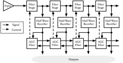
Figure 65 – Cascade structure and smoothing network for the PZFC.

The various parameters of the PZFC can be chosen to give the best fit to various pieces of physiological and psychophysical data. These fits are presented in a later section, but throughout this section I will refer to the 'baseline' parameters, which are the parameters used before fitting. This is the parameter set used in the experiments described in section 2 of chapter 4.

The PZFC was developed by Dick Lyon, based on his previous work on cascade filterbanks. I developed versions of the PZFC filterbank for AIM-MAT and AIM-C, based on Lyon's original implementation.

Pole and zero positions

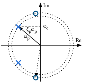
Figure 66 – Diagrammatic representation of the placement of the poles and zeros in the S-plane for the PZFC. The dotted circles show the trajectory of the pole and zero motion as a function of the damping parameter

ξ

.

The pole and zero positions are specified in terms of their natural frequencies ( $ω p$ and $ω z$ , for the pole and zero, respectively) and their damping constants ( $ξ p$ and $ξ z$ ). As the damping is increased from zero, the pole and zero move on a circle in the S-plane. Figure 66 shows the conjugate pole and zero pair; $ω p$ is the natural frequency of the pole, $ω c$ is the instantaneous centre frequency for a given damping, and $ξ p ω p$ gives the pole attenuation (distance from the imaginary axis). The system is described by the following transfer function:

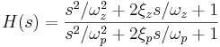
$H(s) = \frac{s^2/\omega_z^2 + 2\xi_z s/\omega_z + 1}{s^2/\omega_p^2 + 2\xi_p s/\omega_p + 1}$

The natural frequencies of the pole and the zero are constants, decreasing from one stage to the next, along a cochlear frequency–place map, or ERB-rate scale. At each stage $ω z$ is fixed at $f_z \times \omega_p$ , where $f z$ is the 'z factor', and is set at 1.4 in the baseline case. The channel density for the filterbank is set by a step factor, which determines the channel density as number of channels per ERB. The channel density is set at 3 channels per ERB in the baseline case. Figure 67 shows the individual filter stages of the PZFC before any adaptation due to the smoothing network, and Figure 68 shows the overall frequency response of the PZFC filterbank at each output.

Figure 67 – PZFC filterbank stages.

Figure 68 – PZFC filterbank overall response before any level modification due to the AGC network.

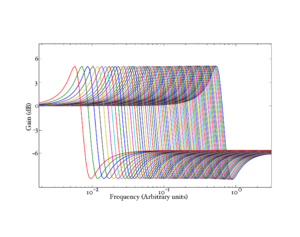
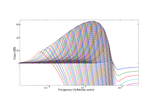
Two parameters, $P damp$ and $Z damp$ , set the damping factors for the pole and the zero respectively. The pole damping varies dynamically as $ξ p = P damp (1 + AGC)$ (where AGC is a function of the state of the automatic gain control circuit described below) and the $Z damp$ parameter sets the zero damping directly: $ξ z = Z damp$ . In the baseline case, $P damp$ is set at 0.12 and $Z damp$ is set at 0.2. Figure 69 shows the effect of changing the two damping parameters on the peak of the stage frequency response.

Figure 69 – Effect of modifying the damping parameters on the PZFC frequency response. When

P damp

is varied,

Z damp

is held at 0.2, and when

Z damp

is varied,

P damp

is held at 0.12.

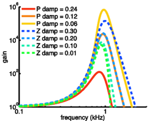
Automatic gain control

The PZFC automatic gain control (AGC) is achieved by a temporal and spatial smoothing network. This network takes the output of all the channels, applies smoothing in both the time and frequency dimensions, and uses both global and the local averages of the filterbank response to affect the pole damping, $ξ p$ at each stage. In Lyon’s implementation, the dynamic smoothing network allows the filterbank to adapt to changes in the input on time scales from the order of a few milliseconds up to hundreds of milliseconds. While it is useful, in practical terms, to ascribe AGC timescales on the order of hundreds of milliseconds to processes in the cochlea, it is not physiologically realistic. Adaptation that occurs on this timescale is likely to originate more centrally.

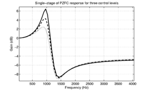
Figure 70 – Impulse response of one of the four sets of parameters in the AGC smoothing network. The activity diffuses out in space and decays exponentially in time.

Figure 71 – PZFC filterbank stage at three different levels

The smoothing network takes the form of a four-stage filtering process. The output of each filter channel is first half-wave rectified and weakly compressed using a cubic nonlinearity. This monopolar signal is then passed through a set of low-pass filters, which have the effect of smoothing the signal. Four first-order filter stages are arranged in parallel, each having one state variable per channel. Each stage has a different time constant, which determines how much the state in a channel should be affected by the current filter output. Spatial smoothing is achieved by coupling the states to their neighbours at adjacent channels --- a simple filter convolves the AGC state for each stage with a three-channel wide triangular window, once per sample. This has the effect of causing the signal in one channel to gradually diffuse out to affect the control parameters in other channels. An application was designed to reveal the spread of adaptation in frequency and time, in preparation for experiments designed to examine the physiological plausibility of the smoothing network, which is unlikely to be symmetric in the cochlea. Figure 70 shows the impulse response of the smoothing network. Note the exponential decay in the centre channel, and the symmetrical diffusion of activity out to more distant channels. Figure 71 shows the response of a single filter stage as the pole position is modified by the AGC system.

The pole dampings in each channel are scaled (increased from their values in quiet) by a factor proportional to the mean of the four AGC stages in that channel. Thus, a sustained high input level in a channel will cause the poles for the associated filterbank stage, and those around it, to move further from the imaginary axis in the S-plane, reducing the gain and sharpness of the combined filter in that channel and those around it. As time passes, this damping effect will propagate to more distant channels, until an equilibrium state is reached. Figure 72 shows the response of the individual filter stages after adaptation to a human /a/ vowel, and Figure 73 shows the overall filterbank response after adaptation. The original response of the filter stages, before adaptation, is seen in Figure 67.

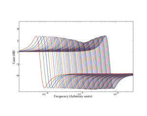
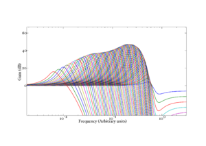
Figure 72 – PZFC filterbank stages after processing several seconds of audio. The AGC network has caused the response of the individual stages to change.

Figure 73 – Overall PZFC filterbank response after processing several seconds of audio.

The smoothing network is intended to simulate the active mechanism in the cochlea, whereby the outer hair cells (OHCs) dynamically modify the response of the basilar membrane to a stimulus. The cascade architecture of the PZFC mimics transmission-line architecture of the cochlea, in which the incoming wave travels along a medium with slowly-changing properties. This makes the filterbank a more physiologically plausible model of the processing actually occurring in the cochlea. However, as it stands, the AGC mechanism does not model the physiological system particularly accurately. There is currently no known physiological analogue for a mechanism by which gain control information propagates symmetrically out from a point on the basilar membrane to points both higher and lower in frequency.

Fitting the PZFC to human masking data

Two studies, by Baker et al. (1998) and Glasberg and Moore (2000), measured the threshold in humans for detection of a sinusoid in asymmetric notched noise. Both studies covered a large range of frequencies and levels, spanning most of the normal range of hearing. The data from these studies were used by Patterson et al. (2003) to fit a set of parameters for the cGC filter; they describe a fitting technique for auditory filters, based on the 'polyfit' procedure which was used by Baker et al. to fit roex functions to their original data.

The polyfit procedure attempts to fit a frequency-domain auditory filter to a set of masking data obtained with a single probe frequency at a wide range of probe levels. Patterson et al. (2003) extended the technique to allow fitting to data from multiple probe frequencies simultaneously. The updated procedure makes the assumption that the variation of any of the filter parameters with probe frequency can be represented as a linear function of the frequency in ERBs.

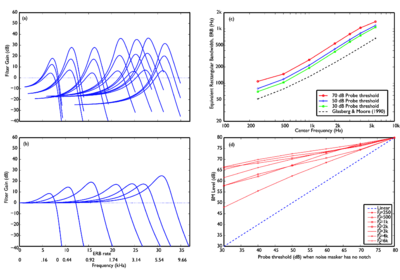
Figure 74 – Results of a fit of human masking data to a PZFC with 10 free parameters. (Fit 517 from Figure 75). Panel (a) shows the absolute frequency response of the filters as a function of stimulus level. Panel (b) shows the responses at a single stimulus level with the filter tail tied at 0dB gain. Panel (c) shows the equivalent rectangular bandwidth of the filter (ERB) as a function of centre frequency, for three different probe levels. Panel (d) shows the input-output curve for the filterbank as a function of level. In this panel, the dotted line shows a linear response, and the red lines correspond to the different filter centre frequencies.

In the case of the gammachirp filter, the procedure fits a total of five filter parameters with constants or linear functions. The total number of free parameters used for the filterbank can be set by choosing how many of the filter parameters to represent as constants, and how many as linear functions. A further two non-filter parameters are fitted with parabolic functions, rather than linear functions. These non-filter parameters, $K$ and $P 0$ , define the efficiency of the detection mechanism following the cochlear filter, and the lower limit on the threshold respectively.

Lyon used the fitting routines employed by Patterson et al. to fit the PZFC to human masking data. In order to fit the human masking data of Baker et al. and Glasberg and Moore with the PZFC, a number of modifications were made to the fitting technique described by Patterson et al.. K, the measure of detection mechanism efficiency, was removed from the search space as it can be determined from the other parameters. In addition to this, search over centre frequencies was made near-continuous to minimise confusion of estimated gradients, and the robustness in small-signal behaviour was improved.

Figure 74 shows the results of fitting the PZFC to the masking data of Baker et al. (1998) and Glasberg and Moore (2000). The four panels show various aspects of the response of the filterbank. The top-left panel shows the absolute frequency response of the filters as a function of stimulus level. The bottom-left panel shows the responses with the filter tail tied at 0dB gain. The filter gain increases in the low ERB range, and levels off in the higher ERB range. The top-right panel shows the equivalent rectangular bandwidth of the filter (ERB) as a function of centre frequency, for three different probe levels. Filter bandwidth is seen to increase as a function of level, but even at the lowest level, the bandwidth is above that estimated with the gammatone. The bottom-right panel shows the input-output curve for the filterbank as a function of level. In this panel, the dotted line shows a linear response, and the red lines correspond to the different filter centre frequencies.

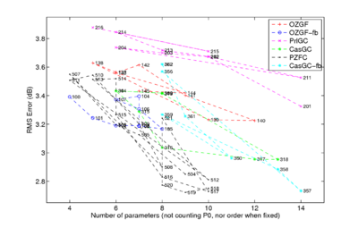
Figure 75 – RMS fitting error as a function of number of parameters, for a number of filter types. This plot was generated using Lyon's updated filter fitting routines. `OZGF' is the one-zero gammatone filterbank and `PrlGC' and `CasGC' are parallel and cascade gammachirp filterbanks respectively. In the `-fb' variants, feedback from the output in a filter channel controls the gain of the filterbank in that channel (a potentially unstable configuration).

Figure 75 shows the RMS fitting error as a function of number of parameters, for a number of filter types. The plot was generated using Lyon's updated filter fitting routines, and it shows that the PZFC can fit the human masking data more accurately with fewer parameters than the parallel and cascade versions of the compressive gammachirp filterbank.

Figure 76 --- Results from fitting the compressive gammachirp filterbank to human masking data. The figure is taken from Unoki et al. (2006). Panel (a) shows the absolute frequency response of the filters as a function of stimulus level. Panel (b) shows the responses of the component filters of the cGC. The solid lines show the response of the passive gammachirp filter, and the dotted lines show the response of the active filter. Panel (c) shows the equivalent rectangular bandwidth of the filter (ERB) as a function of centre frequency, for three different probe levels. Panel (d) shows the input-output curve for the filterbank as a function of level for a range of different centre frequencies,

P g c p

is the output level of the passive gammachirp filter.

Figure 76 shows the characteristics of the compressive gammachirp (cGC) filterbank in the same format as presented in Figure 74 for the PZFC. This allows for comparison of the two filterbank responses in a greater level of detail. The cGC is the filterbank upon which the dynamic compressive gammachirp (dcGC) is based. While the results for the PZFC and the cGC are similar, there are some differences between the responses of the two filterbanks. In panel (a), the cGC is seen to have a steeper high side to the filter. Panel (c) shows the bandwidth as a function of filter centre frequency. In both cases, the filter bandwidths are wider for louder signals, as would be expected, and they both follow the form of the measured ERB function in humans well. However, the PZFC has a smaller range of variation in bandwidth as a function of level. The compression functions (shown in panel (d)) show a smaller spread as a function of frequency in the PZFC compared to the cGC. The PZFC also has a less well-organised structure to the compression functions than the cGC. Overall, the PZFC fits the masking data well using fewer parameters than the dcGC, but the compression functions are not as orderly, and the upper side of the PZFC is probably not quite as sharp as it should be.

The dynamic compressive gammachirp

The dynamic compressive gammachirp (dcGC) filterbank is a parallel-architecture filterbank with a cascaded control channel (Irino and Patterson, 2006).

It was demonstrated by Irino and Unoki (1999) and Unoki et al. (2001) that the gammachirp filter can be decomposed into a cascade of a gammatone filter and an asymmetric compensation function that controls the effective value of the chirp parameter, $c$ . Indeed, the chirp parameter of any gammachirp filter can be modified by cascading it with an asymmetric compensation function of the correct form. Such a cascade architecture is used in the dcGC filterbank to dynamically modify the chirp parameter of each filterbank stage independently as a function of the input signal. Figure 77 shows the response of the passive gammachirp filter, the high-pass asymmetric compensation filter for different levels, and the response of the combined compressive gammachirp (cGC) filter.

Figure 77 --- Response of the passive gammachirp filter (pGC), the high-pass asymmetry function (HP-AF), and the compressive gammachirp (cGC) filter for probe levels of 30, 40, 50, 60, and 70 dB. Figure taken from Irino and Patterson (2006) used with permission of the authors.

In the first, passive, stage, the incoming signal is passed through a gammachirp filterbank that has no level-dependence. In the active part, the output of each channel is passed through a dynamically controlled asymmetric compensation filter that modifies the bandwidth and peak frequency of the overall composite filter. The parameters of this active asymmetric compensation filter are controlled by the processed output of a higher-frequency channel in the filterbank. The control parameter is an estimate of the instantaneous output level of the control channel. This level estimate is calculated from a linear combination of the original passive filter output, and the output of an asymmetric compensation filter with fixed parameters acting on that output.

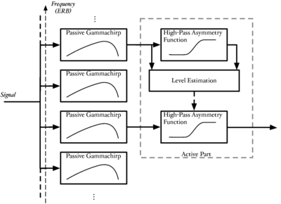
Figure 78 -- Architecture of the dcGC filterbank

Figure 78 shows the architecture of the dcGC. The active part is shown for only one channel of the filterbank. The solid lines show the path of the signal through the filterbank, and the dotted line shows the control parameter for the active high-pass asymmetry function. Since the control parameter is updated instantaneously (on a sample-by-sample basis in the digital implementation), the filterbank exhibits extremely fast-acting compression at sub-millisecond timescales. This compression allows the filterbank to compress the individual glottal cycles in human vocalisations, while allowing the resonance that follows them to ring. Thus the dcGC can effectively reduce the dynamic range of an input signal, and facilitate the analysis of the resonance information following a pulse. The various parameters of the dcGC filterbank have been fitted to human masking data over several studies (Unoki et al., 2001; Irino and Patterson, 2001; Patterson et al., 2003; Irino and Patterson, 2006; Unoki et al., 2006).

Comparing the PZFC and the dcGC

The architecture of the dcGC is fundamentally different from that of the PZFC. Whereas the dcGC is essentially a parallel filterbank wherein all filters get the same input signal, the PZFC is a cascade filterbank with each filter fed by the one before it in the cascade. A further major difference is in the flow of activity in the AGC circuits. In the PZFC, activity from a filter spreads out in both directions symmetrically to influence the response of both lower and higher frequency filters. In the dcGC, the activity in each channel affects only one other channel in the filterbank, as the control signal always flows from a higher-frequency channel to a lower-frequency channel.

The major benefits of the PZFC are that it is efficient to implement, either in hardware or in software (because it consists of a simple cascade of second-order filters) and that it accurately models the travelling wave in the cochlea. By contrast, the dcGC, while still efficient, uses a fourth-order filter cascaded with a set of four second-order asymmetry functions for the signal path in each stage, and another four second-order asymmetry functions for the level estimation path. However, the dcGC has a sound theoretical basis from the point of view of the optimal processing of pulse-resonance sounds; the automatic gain control bears more resemblance to that seen in the cochlea, and it has been well tested in several models. It is for these last two reasons that the PZFC needs more testing and improving before it can be considered as good as the dcGC for modelling auditory processing.

A further problem with the PZFC is that, in the design detailed in this thesis, it is not able to successfully model the data on zero-crossings of the auditory filter response. Studies have shown that the chirp rate of the auditory filter does not vary with the level of the stimulus (Carney et al., 1999), and so the zero-crossings of the impulse response should remain fixed in time as the level changes. However, because the AGC causes the poles of the filter to move in circular trajectories in the S-plane, the zero-crossings of the PZFC impulse response do shift with level. Recently, Lyon (personal communication) has shown that the positions of the zero crossings can be fixed by making the poles move parallel to the real axis, but details of this change are not currently available.

Figure 79 --- `Cochleagrams' of the output of the PZFC, dcGC and gammatone filterbanks for the word `washwater' spoken by a woman. The level in each plot is scaled such that the darkest greyscale value corresponds to the highest output level for each filterbank, and the greyscale level decays from there to zero for pure white. This allows for comparison of the relative dynamic range of each of the filterbanks.

The main benefits of a compressive filterbank come from its ability to actively and quickly compress the pulses in a pulse-resonance sound, and then to recover quickly in order to retain the resonance information that follows. Figure 79 shows 'cochleagrams' for the word 'washwater' after processing through the PZFC, dcGC and gammatone filterbanks. A 'cochleagram' has the same dimensions as the spectrogram, but the output is continuous in each filter channel, unlike the spectrogram where the output is quantised into 'frames' by the window time-step. No external compression was applied to the output of the filterbanks. The dcGC and PZFC filterbanks compress the output into a smaller dynamic range than the simple gammatone filterbank. The dcGC is particularly effective in bringing up the level of the formants relative to the glottal pulses for the voiced sections. However the PZFC is better at enhancing the level of the unvoiced sections, particularity the 'sh' sound between about 200 and 360ms. These effects are likely to be due to the different time constants employed in the gain control circuits of the two filterbanks. The dcGC has very fast-acting compression, but no time constants that are longer than a few milliseconds. This means that it is very effective in compressing the glottal pulses, but it does not have much effect on the longer-term dynamics of the stimulus. The PZFC, by contrast, has AGC time constants up to the order of hundreds of milliseconds, and so is able to affect the relative level of the output on syllable-length timescales. From this, it seems that there may be a trade-off between fast-acting compression and longer-term gain control.

Figure 80 --- `Cochleagrams' of the output of the PZFC, dcGC and gammatone filterbanks for a two-formant synthetic vowel. The level of the stimulus was ramped down linearly (on a dB scale) from a maximum to -48dB over the course of one second. Scaling is as in Figure 79 so that dynamic range can be compared.

Figure 81 --- `Cochleagrams' of the output of the PZFC, dcGC and gammatone filterbanks for a two-formant synthetic vowel. The level of the stimulus was ramped up linearly (on a dB scale) from a minimum of -48dB to the maximum amplitude possible over the course of one second. Scaling is as in Figure 79 so that dynamic range can be compared.

Figure 80 and Figure 81 show the responses of the PZFC, dcGC and gammatone filterbanks to a two-formant synthetic vowel that changes rapidly in level over the course of a second. In both cases, the PZFC compresses the output most strongly, leading to the longest visible patterns of activity in the image.

In the remainder of this section, the detection of periodicity in various stimuli is used to compare the temporal dynamics of the dcGC and the PZFC filterbanks. It seems that dynamic, compressive filterbanks produce better features for modelling pitch strength within time-domain models such as AIM. Specifically, use of the PZFC or the dcGC filterbank within AIM was found to provide a more pronounced peak in the temporal profile of the auditory image than the standard gammatone filterbank, for complex sounds like iterated rippled noise (IRN).

The mechanism that sharpens the peak is not immediately clear, but what is clear is that time-varying compression is an important factor in the processing of these stimuli. In the following sections I detail a number of experiments performed to judge the ability of an AIM-based model with a dcGC or PZFC filterbank to detect the dominant periodicity in these stimuli.

Stimuli

Iterated rippled noise

Iterated rippled noise (IRN) is a stimulus that is frequently used as a test of auditory models. It has a power spectrum that resembles that of a noise, but gives rise to a pitch percept in the auditory system. IRN is created by repeatedly time-shifting and summing a block of white noise. This has the effect of adding a repeating temporal structure to the noise. After several iterations of this delay-and-sum process, a weak pitch is observed in the stimulus, which gradually becomes stronger as more iterations are performed. Figure 82 shows a circuit for generating IRN by repeatedly adding a delayed version of the waveform to itself. In the spectral domain, the delay-and-sum process adds a small `ripple' to the spectrum of the sound, which gives it a weak harmonic structure. Repeated iterations of the delay-and-sum process enhance the depth of the ripple.

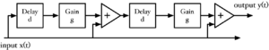
Figure 82 --- Circuit for generating IRN. Two iterations shown. Figure redrawn from Yost et al. (1996).

The phenomenon of a repeated noise giving rise to a pitch was first reported by Huygens (1693), who observed that a pitch was present in the sound of a fountain opposite a flight of stone steps. Huygens determined that the pitch of the sound was equivalent to that generated by a small organ pipe of the same length as an individual step. The multiple reflections of the fountain noise from the vertical surfaces of the staircase had the effect of summing multiple copies of the noise waveform, giving rise to what we would now call IRN. A similar effect has been observed in Mexican step pyramids, where a handclap elicits a chirping noise reflected from the vertical surfaces (Bilsen, 2006).

IRN is an excellent stimulus for testing the characteristics of filterbanks and strobed temporal integration mechanisms (see chapter 3). IRN has been a challenging stimulus for spectral models of pitch perception (Yost and Hill, 1979). Pitch extraction in AIM is based on the temporal fine structure of a sound, and pitch strength corresponds to the peak height in the temporal profile of the SAI. Thus, the auditory image model gives a specific way of modelling the pitch strength of stimuli which lack a strong spectral structure.

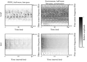
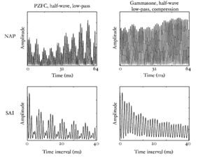
Figure 83 --- NAPs and SAIs generated from a 16-iteration IRN stimulus using the PZFC and gammatone filterbanks. The PZFC output is half-wave rectified and lowpass filtered (hl), the gammatone filterbank output is logarithmically compressed as well as being half-wave rectified and low-pass filtered (hcl).

Figure 84 --- The output of the 770Hz channel in Figure 83

Figure 83 and Figure 84 show the response of the PZFC and gammatone filterbanks to the same IRN stimulus, and the resulting SAIs generated from the signal. The pitch feature in the SAI of the PZFC is better defined than that in the SAI of the simple gammatone filterbank.

Measures of pitch strength

In order to further investigate the pitch strengths produced by the three filterbanks it is necessary to have some absolute measure of pitch strength in the SAI temporal profile. Ives and Patterson (2008) developed just such a measure, which estimates the pitch strength of harmonic complexes from the vertical ridge of activity that appears in the SAI at the time interval associated with the pitch. Their measure was simple: they computed the temporal profile and found the largest peak in the region of the time-interval associated with the pitch. They then found the two local minima immediately adjacent to this peak, and took the mean of the levels of the two minima. This mean minimum level was then subtracted from the level of the maximum to get a local peak height. This was taken as the pitch strength. Ives and Patterson (2008) used this to study the relative pitch strength from a model using the dcGC filterbank and the gammatone filter.

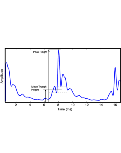
Figure 85 --- Pitch strength measure used by Ives and Patterson (2008). This figure is modelled on figure 6 from Ives and Patterson (2008).

This pitch strength measure was used to estimate pitch strength from the temporal profiles of auditory images. The technique of Ives and Patterson (2008) was modified slightly in two ways. Since the repetition rate of the stimuli was already known, the search space for a local maximum in the SAI temporal profile was limited to a region around the fundamental. The search space for a maximum was 1.5ms each side of the repetition rate. In order to compare the output of different filterbanks, the SAI temporal profiles were all normalised such that the local maximum in the region of the pitch was at 1. Since the SAI profiles were truncated at 0.5ms (the standard parameter for the ti2003 AIM-MAT module), this led in many cases to the peak due to the repetition rate being the highest point in the temporal profile. However, in some cases, particularly for the PZFC, the decay rate in the SAI profile after the zero-lag peak was such that the SAI profile was at a higher value near the zero-lag line. This effect is visible in some panels of Figure 89, where the temporal profile is 'clipped' at the low-lag end. Figure 85 shows how the measure is calculated from the peak and adjacent troughs.

Comparison to human pitch perception

The normalised pitch-strength measured for IRN stimuli was compared with the pitch strength measured for IRN in perceptual experiments. Patterson et al. (1996) performed a series of experiments on the human perception of IRN by comparing the pitch strength of IRN stimuli and tonal stimuli masked with noise (Yost, 1996; Yost et al., 1998; Patterson et al., 2000; Handel and Patterson, 2000). Subjects compared IRN with different numbers of iterations to a tonal stimulus (256-iteration IRN with a 16ms delay time) masked with noise. Subjects were asked to select the stimulus with the stronger pitch strength as the SNR of the noise-masked tonal stimulus was changed. In their experiments two conditions were tested, in which the stimuli were high-pass filtered with a cutoff frequency of either 50Hz or 800Hz. The 800Hz filter condition was designed to exclude the resolved harmonics from the stimulus. The pitch strength measure described above was used to model the data of Patterson et al. (1996), using the techniques described in that study. The original results from the perceptual experiment are plotted in Figure 86, the predictions made by Patterson and Yost's model are shown in figure Figure 87 and the predictions made using the current measure on an SAI made using a PZFC filterbank are plotted in Figure 88. In each case, the horizontal axis is the tone to noise ratio, and the vertical axis is the predicted proportion of the time that the standard noise-masked tonal stimulus was picked as having a higher pitch strength than the IRN stimulus. In practice the results of Patterson et al. (1996) did not show much difference between the 50Hz and 800Hz condition, and a similar result was seen when using the pitch strength measure described here, so only the more challenging 800Hz condition is compared.

Figure 86 --- Psychometric functions for test IRNs from Patterson et al. (1996) (Figure 1).

Figure 87 --- Pitch strength predictions for the perception of IRN in noise, from the autocorrelation model ofPatterson et al. (1996) (Figure 5).

Figure 88 --- Predictions (dashed lines) of the perceptual data of Patterson et al. (1996) (solid lines) made using the normalised pitch strength measure employed in the experiments in this section applied to auditory images generated with a PZFC filterbank. The results follow the same pattern as the perceptual results reported in Patterson et al. (1996), but the measure is slightly noisier than the model used in that paper.

The predictions made by the normalized pitch strength measure in Figure 88 have the same form as the perceptual results reported in Patterson et al. (1996). The form of the results for the other filterbanks is similar. The curves predicted by this model are a little noisier than those from the model of Patterson et al. (1996), but the model has the advantage of being normalised making it easier to compare results across filterbanks when their output levels differ.

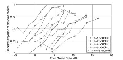
Experiments

Comparing pitch strength estimates using IRN

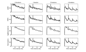
Figure 89 --- SAI temporal profiles generated with four different sets of filterbank / NAP parameters for an IRN stimulus with a delay of 8ms. The leftmost column shows the SAI temporal profile for a zero-iteration IRN, which is a noise. The remaining columns show the response for 1, 2, and 4 iteration IRN stimuli. For the 1, 2 and 4 iteration IRN, a peak is expected in the temporal profile at 8ms time interval.

Figure 89 shows SAI temporal profiles generated with the dcGC, the PZFC and the gammatone filterbank with and without logarithmic compression for IRN stimuli. The profiles for the zero-iteration IRN (just noise) show little temporal structure, as we would expect. It is clear from inspection that the gammatone filterbank with logarithmic compression produces profiles in which the peak in the profile which corresponds to the perceived pitch is much less strong than for the other filterbanks. For comparison, the results from the gammatone filterbank without logarithmic compression are included. The pitch strength estimates are stronger than for the log-compressed gammatone, but the linear gammatone is not a physiologically reasonable auditory filter model as it has no compression, and it is included in these experiments only for comparison with the other compressive filterbanks.

While the dcGC might be considered to give slightly higher pitch strength estimates based on the data in the figure, there is not any clearly visible difference between the PZFC, the dcGC and the linear gammatone models.

Auditory images were generated from IRN stimuli with 0, 1, 2 and 4 iterations, as described above. The IRN stimuli (specifically IRNo, see Yost et al. (1996)) were generated using the `gen\_IRNo' function in AIM-MAT, and were used to assess the effect of overall pitch saliency on the pitch strength measures extracted from the SAI. The IRN was generated with a delay of 8ms, leading to a 125Hz pitch in the output. The output was band pass filtered with a pass band between 500Hz and 2kHz. The pass band was ramped up over 200Hz and down over 1.6kHz using a raised cosine window; therefore the region of the spectrum containing energy went from 300Hz to 3.6kHz. This bandpass filtering serves to remove the fundamental and second harmonic of the pitch period from the spectrum completely.

Results

<tablenameRef name="irn_results_table"/> shows the mean results from application of the pitch strength estimation algorithm to 20 randomly generated IRN stimuli using the above parameters. It is clear from these results that the dcGC gives rise to a considerably stronger pitch feature in the temporal profile of an IRN stimulus than do the other filterbanks. While the pitch feature from the PZFC is stronger than that from the log(gammatone) filterbank, the results are on a par with the results from the linear gammatone. Standard deviations for the pitch strength measures are given in brackets after each value.

<tablename name="irn_results_table"/> Mean pitch strength estimates for 20 randomly-generated IRN stimuli using four filterbanks and 1, 2 and 4 iterations when generating the IRN.
	dcGC	PZFC	log(gammatone)	gammatone
1 Iteration	0.553 (0.055)	0.441 (0.056)	0.297 (0.040)	0.421 (0.044)
2 Iterations	0.566 (0.089)	0.461 (0.056)	0.313 (0.049)	0.432 (0.061)
4 Iterations	0.633 (0.051)	0.504 (0.055)	0.342 (0.058)	0.502 (0.049)

The results suggest that the processing performed by the dcGC is fundamentally different to that performed by the PZFC for these stimuli. In order to determine why performance with the PZFC is inferior to that with the dcGC, we now turn to a deterministic signal to perform several experiments on the AGC of the PZFC.

Harmonic complexes

Clara Suied generated an interesting set of bandpass-filtered harmonic complexes for an experiment on the perception of pitch height. These stimuli were 125Hz harmonic tones, in which the 9th harmonic was the lowest component. The envelope of the amplitude spectrum was flat in a pass band which was six ERBs wide. This is a stimulus design suggested by Krumbholz et al. (2000). Above the flat pass band, the envelope of the amplitude spectrum was smoothly attenuated to zero with a quarter-cycle cosine envelope function. Below the passband, the envelope was simiarly raised from zero with a quarter-cycle sine envelope. The width of the envelope function below the passband was 2 ERBs, and above the passband it was 4 ERBs.

In the experiments below, Suied's baseline stimulus is used to experiment with modifications to the PZFC automatic gain control (AGC). For quantitative measurement of the effect of changes on the PZFC parameters, these stimuli are easier to deal with than IRN because IRN is inherently a noisy stimulus, and it would be necessary to average over stimuli to achieve measurements that can be used for comparison.

Modified PZFC AGC parameters

The base harmonic complex stimulus (0 degrees phase shift, no spectral envelope shift) was used to further assess the effect of changing the PZFC parameters on the pitch strength measures produced with that filterbank.

Temporal smoothing in the PZFC AGC is implemented with a smoothing filter that is convolved with the AGC activity once per sample. The filter is three channels wide and in the default configuration is triangular in form. Choosing the relative levels of the three coefficients changes the way in which energy is distributed in the smoothing process.

The default configuration of the smoothing filter has the coefficients 0.3, 0.4 and 0.3 (left, centre and right). The parameters sum to unity in order to maintain the overall activity within the AGC smoothing network. When these coefficients are convolved with the smoothing network activity in each channel, the activity spreads out equally to higher and lower frequencies. This default configuration is tested as parameter set 0 in the experiments below.

To force the activity to spread asymmetrically, the experiments above were repeated with several different configurations of the AGC parameters. These configurations are designed to be weakly and strongly asymmetrical, preferentially pushing activity either to lower frequencies (as in the dcGC) or to higher frequencies. The configurations of the parameters, along with the pitch strength estimates, are shown in <tablenameRef name="pzfc_agc_coeffs"/> as parameter sets 1 to 6. In the case of parameter sets 5 and 6, the activity does not diffuse along the spatial dimension but is actively 'transported', since one of the off-centre coefficients is larger than the central coefficient.

The AGC also has four temporal constants $ε n$ where $n$ is from 1 to 4. These parameters determine the decay rate of activity in each of the four AGC channels. The activity in the AGC channel is attenuated by a factor of $1 - ε n$ at each time step, and the current activity from the filterbank channel is added with weight $ε n$ . In channels with a large constant, activity in a channel at a certain time dies away quickly. Conversely, a small decay constant leads to activity affecting the AGC state for a longer period of time.

The default decay constants for the PZFC AGC are 0.0064, 0.0016, 0.0004 and 0.0001 per sample. At a sample rate of 44kHz, these constants correspond to activity half-lives of roughly 2ms, 10ms, 40ms and 160ms. These constants can be modified to change the integration time of the AGC.

Several alternative sets of constants were tried to test the temporal dynamics of the filterbank. Since none of the AGC parameters were actually fitted when the PZFC was fitted to the masking data, we are free to choose values which give the best temporal dynamics for the filterbank. The modified AGC coefficients, and pitch strength estimates, are shown in lines 7 to 11 of <tablenameRef name="pzfc_agc_coeffs"/>.

<tablename name="pzfc_agc_coeffs"/> Tested configurations of the PZFC spatial and temporal smoothing filters, and measured pitch strength for a harmonic complex using these parameters. Spatial coefficients are from high frequency to low frequency.
	Spatial	$ε n$	Pitch strength
0	0.3, 0.4, 0.3	0.0064, 0.0016, 0.0004, 0.0001	0.698
1	0.1, 0.5, 0.4	0.0064, 0.0016, 0.0004, 0.0001	0.695
2	0.4, 0.5, 0.1	0.0064, 0.0016, 0.0004, 0.0001	0.702
3	0.0, 0.5, 0.5	0.0064, 0.0016, 0.0004, 0.0001	0.713
4	0.5, 0.5, 0.0	0.0064, 0.0016, 0.0004, 0.0001	0.716
5	0.0, 0.2, 0.8	0.0064, 0.0016, 0.0004, 0.0001	0.777
6	0.8, 0.2, 0.0	0.0064, 0.0016, 0.0004, 0.0001	0.691
7	0.3, 0.4, 0.3	0.0128, 0.0032, 0.0008, 0.0002	0.683
8	0.3, 0.4, 0.3	0.0256, 0.0064, 0.0016, 0.0004	0.682
9	0.3, 0.4, 0.3	0.4096, 0.2048, 0.0512, 0.0128	0.858
10	0.3, 0.4, 0.3	0.4096, 0.0128, 0.0128, 0.0128	0.836
11	0.3, 0.4, 0.3	0.4096, 0.4096, 0.4096, 0.4096	0.874

In order to compare the PZFC results against the other filterbanks, the baseline measurements of pitch strength for the default configurations of the other filterbanks are shown in <tablenameRef name="hc_other_table"/>.

<tablename name="hc_other_table"/> Measured pitch strength for a harmonic complex using the dcGC and gammatone filterbanks.
dcGC	log(gammatone)	linear gammatone
0.873	0.535	0.661

Figure 90, and <tablenameRef name="pzfc_agc_coeffs"/>, show the pitch strength estimates for the harmonic complex stimulus with the baseline PZFC parameters and the 11 sets of modified parameters. Modification of both the spatial AGC parameters and the temporal AGC parameters can lead to higher pitch strength estimates than those produced with the baseline configuration. Interestingly, the largest improvement occurs when the time constants are much larger than the default values (leading to far shorter half-lives for the AGC) and when the range of the half-lives is reduced. The faster time constants are more like those seen in the dcGC filterbank. The largest pitch strength estimate is achieved when the AGC employs the shortest time constants, and it is larger than that for the dcGC operating on the same stimulus. Modification of the spatial smoothing constants has a smaller effect on the pitch strength estimate, but the case where the coefficients push the activity strongly from higher-frequency channels to lower-frequency channels has the greatest effect. This is again what we would expect -- activity in higher-frequency channels affects activity in lower-frequency channels, but not vice versa.

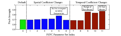
Figure 90 --- Pitch strength measures from SAI profiles generated from a harmonic complex. The PZFC filterbank was used in all cases, and the automatic gain control coefficients of the PZFC were varied.

Figure 91 --- Cochleagrams for the word 'washwater' using the baseline PZFC (top) and PZFC parameter sets 8 and 9 (faster AGC time constants) (middle and bottom). Scaling is as in Figure 79 so that dynamic range can be compared.

Figure 91 shows cochleagrams for the baseline PZFC parameter set (top) and the parameter sets 8 and 9 (middle and bottom) for the word 'washwater' once again. Parameter set 9 produced a considerably higher pitch strength estimate than parameter set 8 for the harmonic complex stimulus. In the cochleagrams, parameter set 9 is seen to apply more compression to the signal than the baseline parameters or parameter set 8. The upper formants of the vowel sounds are now more clearly visible. Although this effect of increased compression has a positive effect on pitch strength, it may in fact degrade the output signal, giving low-level features too much weight relative to high-level ones. In the 'sh' sound, there is considerable activity visible at low frequency, which does not reflect the energy distribution in the input well.

While it is interesting to see that making the AGC of the PZFC react faster has a positive effect in increasing its ability to resolve pitches, it is not immediately clear why this should be the case. Since the effect of fast-acting compression should be to compress glottal-pulses in the input stimulus, one might expect the pitch strength to go down as the speed of the compression was increased. A full study of this effect is beyond the immediate scope of this research, but it is something that I intend to study more fully in the future.

Further work and Conclusions

In this section I have introduced Lyon's pole-zero filter cascade (PZFC) filterbank as an efficient compressive auditory filterbank which can model well the masking data from humans, and compared it to another compressive filterbank, the dynamic compressive gammachirp (dcGC). The PZFC filterbank was implemented in AIM-C and AIM-MAT, using the original implementation by Lyon as a basis. It was tested against dcGC filterbank and the linear and log-compressed gammatone filterbanks in two pitch-strength determination tasks. The PZFC was found to be computationally efficient and to have compression characteristics that enable it to extract pitch from stimuli that have traditionally been challenging to pitch determination algorithms. A number of modifications were made to the automatic gain control (AGC) parameters of the PZFC filterbank to improve its abilities in this regard. These experiments point the way for future work on optimising the PZFC.

The PZFC is an efficient and accurate implementation of an auditory filterbank, and it has the benefit of being based firmly in the fluid dynamics of the cochlea. However, the dcGC filterbank is a better-established filterbank which has been rigorously tested against a variety of psychophysical and physiological data. Currently, the dcGC is better tuned to these data than the PZFC. However, the experiments above demonstrate that it is possible to manipulate parameters of the PZFC AGC to give better performance on certain real-world tasks. Using a similar analysis framework and a wider range of stimuli, it is likely that the PZFC's parameters can be tuned to further improve its performance.

One interesting approach to this problem would be to modify the AGC of the PZFC so that its architecture was more like that of the dcGC. The AGC activity could be shifted so that the state of an AGC stage which takes input from one frequency is used to affect the PZFC filter stage at a lower frequency. This would align the PZFC AGC architecture more closely with models of compression in the cochlea.

The experiments presented in this chapter do not, on their own, justify the use of a compressive filterbank in a machine hearing system. However, they provide an insight into the utility of compressive filterbanks in the processing of stimuli in which the temporal fine structure is important.

A potential continuation of this work would be to use the compressive filterbanks described above in combination with the features generated from the Gaussian mixture model used in the earlier chapters of this thesis. Preliminary experiments to this end, which directly swapped the gammatone filterbank for the PZFC filterbank, led to recognition results which were significantly worse than the results gained with the gammatone filterbank. However the exact parameters of the Gaussian fitting procedure were tuned to the output of a simple gammatone filterbank and these parameters were not modified in the initial experiments. The tuning of these parameters for use with the PZFC and dcGC filterbanks, ideally using a complete search of the parameter space for the Gaussian fitting system, is another potential direction for future work.

While tuning of the AGC circuits of the PZFC, and evaluation of compressive filterbanks with a speech recognition task are probably both worthy of further study, an outstanding opportunity to work with auditory features on a much larger scale suddenly arose in the autumn of 2008. The research team of Dick Lyon at Google had been investigating the use of MFCC features in a large-scale sound effects recognition task, making use of the PAMIR machine learning system which is optimized for use on large datasets. The team was working to extend the model to work with features generated from a version of the auditory image. I was invited to join the team for an internship, working with them on the evaluation of auditory features within the sound effects ranking task.

The system developed at Google was based on the PZFC filterbank and the strobed temporal integration system developed by Dick Lyon and discussed in chapter 3. The speed of the PZFC makes it possible to generate auditory features within a large-scale systems. The efficiency of the filter cascade architecture and the AGC network means that it can provide compressive filtering with not much more computation than a linear gammatone filterbank. This in turn makes it possible for the system to scale to datasets of the size required in Internet search tasks.

Footnotes

Content-based Audio Search

In the previous chapters of this thesis I have developed various parts of an complete system for generating and using features from an auditory model in content-based audio analysis tasks. Having worked on these various individual sections, I was lucky enough to be able to work with a team of researchers at Google, developing an integrated machine hearing system based on auditory images. This system combines variants of the various stages of processing studied in the previous sections into a complete content-based audio search system. The system uses sparse features computed from the SAI, and learns a mapping from these audio feature vectors to a sparse feature vector representing words associated with the sound. In the experiments, two versions of the SAI are used: the 'Lyon-SAI' and the 'AIM-SAI'. The AIM-SAI uses the same combination of strobed temporal integration and image stabilisation as developed in chapter 3, and employed in the syllable recognition experiments in chapter 4. The Lyon-SAI uses the 'Lyon' strobe mechanism discussed in chapter 3, and a slightly different strobed temporal integration process.

Content-based audio search

Note:

The work in this section was performed in collaboration with Richard F. Lyon, Martin Rehn, Gal Chechik and Samy Bengio. Preliminary results were presented in Rehn, Lyon, Bengio, Walters and Chechik (2009). The complete study was published in Lyon, Rehn, Bengio, Walters and Chechik (2010).

Introduction

This study was undertaken as part of the 'machine hearing' research effort at Google. The team at Google defines machine hearing research as developing 'systems that can process, identify and classify the full range of sounds that people are exposed to'.

Developing such systems requires both efficient and effective algorithms for large-scale machine learning of a range of sound categories, and a representation of the sounds themselves that captures the full range of auditory features that humans use to discriminate and identify different sounds. In this work, we used a content-based audio search task as a method of assessing the quality of two representations of sound: features generated by the auditory model and a simple MFCC representation.

When designing the system, it as important to keep in mind the problem of scalability: the systems used are both effective and efficient, as it is desirable to be able to scale up the system to Internet-sized datasets.

Audio search

Figure 92 – Searching for a Lion's roar using Google

Currently, when searching for sound effects on the Internet, one can either go to a specialised sound effects site, such as Freesound or type a text query into a normal search engine. In either case, the results returned are based not on the content of the audio itself, but rather on metadata associated with the audio. Figure 92 shows the results of typing the query `lion roar' into Google (in June 2008). The results are accurate, but only because the words `lion' and `roar' were found somewhere on the page on which the sound was found.

Content-based search

In the application developed here, the interface is very similar: a user enters a textual search query, and in response is presented with an ordered list of sound documents, ranked by relevance to the query. For instance, a user typing `lion' will receive an ordered set of files, where the top ones should contain sounds of roaring lions. However, in this case, text query terms are associated directly with the content of the audio, and no text annotations or other metadata are used at retrieval time.

At training time, a set of labelled sound documents is used, allowing the system to learn to match the acoustic features of a lion's roar to the text tag `lion', and similarly for a large set of potential sound-related text queries. This allows for the searching of large unlabelled databases of audio by the use of text queries, using only a small labelled dataset for training.

The machine learning system used is called PAMIR -- the 'passive-aggressive model for image retrieval' (Grangier and Bengio, 2008). As its name suggests, it was first designed for content-based image search problems, but is equally well suited to the problem of audio search. PAMIR uses high-dimensional sparse features to represent both the audio input and the text terms describing that input. It then learns a linear mapping from the feature space to the query term space.

Representations of sounds

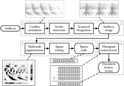
Figure 93 -- Overview of the Machine Hearing system developed at Google Research

In this study, we assessed the difference in performance between MFCC-based features and two forms of SAI-based features. Figure 93 shows the complete system used in the generation of auditory features summarising an audio document. For the SAI-based features, the PZFC filterbank is used as a first stage as it has good compressive properties and is very computationally efficient (1). The two SAI representations (2) differ in the system used for strobed temporal integration. The first system, referred to as the 'Lyon-SAI' uses a simpler strobe detection and temporal integration scheme than is typically used in AIM-based models. The second system is a standard AIM system, based on the sf1992 strobe-detection algorithm (with various improvements discussed in chapter 3 of this thesis) and the ti2003 temporal integration system. The next stage of processing (3) is the sparse coding of the auditory image to produce a high-dimensional feature vector with only a few nonzero elements. This is in accordance with some properties of neural coding (Olshausen and Field, 2004), and has significant computational benefits that allow for the training of very large-scale models. The final stage of encoding (4) is to create a histogram of the sparse-code vectors over the period of interest in the audio. This yields a high-dimensional, but still fairly sparse representation of the audio.

AIM processing

The PZFC filterbank was used as the cochlear model for all the auditory processing in this study. In both cases, the filterbank had 95 channels, spanning a frequency range from 40Hz to 9.3kHz. The NAP was calculated by simple half-wave rectification of the filterbank output. There was no PCP applied.

Lyon-SAI

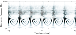
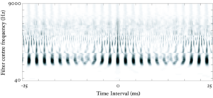
Figure 94 – Example 'Lyon-SAI' for a human vowel.

Figure 95 --- Example 'Lyon-SAI' for a ringing telephone.

Two techniques for generating SAIs were used in this study. The first, known as 'Lyon-SAI' performs strobe detection using multiple overlapping parabolic windows on the NAP signal. The signal in each channel is multiplied pointwise by the windowing function, a parabola of 40ms width. The maximum point in the windowed signal is the strobe point. The window is then shifted by 4ms and the process is repeated. Thus, there is guaranteed to be an average of one strobe point every 4ms, or five per 20ms frame, but it is possible for multiple strobes to occur at one point in the signal, since the windows overlap. Each SAI channel is then calculated as the cross-correlation between the original signal and a signal composed of delta-functions at the identified strobe points. This cross-correlation is accomplished efficiently by simply sliding a piece of the waveform for each channel to move the strobe point to the centre, and adding up the five copies for the five strobe points in the frame. The Lyon-SAI has its zero-lag line at the centre of the time-interval axis and is truncated at ±26.6ms. Figure 94 shows an example of a SAI frame for a human vowel using the Lyon-SAI technique, and for comparison, Figure 95 shows a Lyon-SAI for a ringing telephone. The Lyon-SAI technique is not strobed temporal integration in the sense that it is used in AIM, as the SAI is generated afresh for each frame and there is no naturally occurring decay in the time-interval dimension. However, for practical purposes, the Lyon SAI technique is an effective and efficient method for generating an SAI.

AIM-SAI

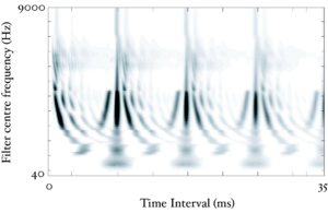
Figure 96 – Example 'AIM-SAI' for a human vowel.

The AIM-SAI as used in this study uses a variant of the local maximum algorithm (see chapter 3) for strobe-detection, and the ti2003 system (as employed in both AIM-MAT and AIM-C) for SAI generation. Figure 96 shows an AIM-SAI generated using this technique. In the variant of the strobe algorithm used here, the strobe threshold starts at zero. When the signal exceeds threshold, a strobe point occurs and the threshold is raised to the level of the signal at the time of the strobe. Following a strobe, the threshold decays linearly to zero over 20ms. The time constant for the decay is set such that the threshold will decay more slowly than the resonance following a pulse, and so the next supra-threshold peak in the signal is likely to have been caused by a new incoming pulse. A 5ms lockout period prevents a strobe from occurring immediately after the previous strobe; this prevents multiple strobes from occurring on a fast-rising section of signal.

The SAI generation is the standard system from ti2003: when a strobe occurs, the signal following the strobe starts to be added into the AIM-SAI buffer, starting from zero time-interval. This process continues for 32ms after the strobe has occurred (leading to an AIM-SAI width of 32ms, which is slightly wider than the Lyon-SAI system described above). As time goes on, more strobes will occur, and these too begin to be added into the buffer. When multiple strobes are active (that is, when more than one strobe has occurred within a 32ms window), the signal following each strobe is weighted by an amount inversely proportional to the number of strobes currently active, before being added to the buffer. This ensures that the overall level of the SAI remains equal to the level of cochlear model output, despite the average strobe rate not being fixed.

`Box cutting' and sparse coding

Figure 97 – 'Box-cutting' part A. Rectangular regions are tiled vertically on the image. The left edges of the rectangles are tied to the zero-lag line. The rectangles overlap by half their heights.

Figure 98 – 'Box-cutting' part B. The rectangle heights are doubled and the tiling process from part A is repeated.

Figure 99 – 'Box-cutting' part C. The width of each rectangle is doubled (with the left edge still pinned to the zero-lag line). When the box width is wider than the remaining space in the image, the box is shifted so the right edge is at the right edge of the SAI.

Figure 100 – Example rectangle sizes. The smallest and largest boxes are shown.

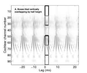
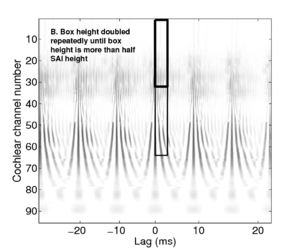
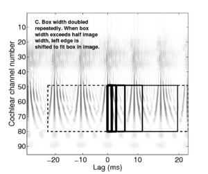
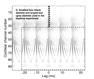
The sparse code used to represent an auditory image is based on identifying patterns that typically appear in a SAI, and then representing the image as a histogram of those patterns that could appear. Patterns that are due to certain sound sources are likely to appear at specific positions in the auditory image. For example, the call of a bird may appear as a band of energy in the higher-frequency channels of the filterbank, whereas a deep musical note from, say, a tuba, would have as a major feature, a set of widely-spaced vertical ridges due to the pulse-rate of the note. At large scales in the SAI, there is information about the pitch and longer-term temporal structure of a sound, and at small scales there is information about the resonances following each pulse. Therefore, instead of looking for patterns only in the whole auditory image, local patterns in different parts of the SAI, and at different scales, are identified. To do this, we define a set of overlapping rectangles of different scales that cover the whole SAI frame, and then the content of each of those rectangles is independently encoded using a separate sparse coder.

Choice of rectangular boxes

The `baseline' rectangle size was chosen to be 16 samples in the lag dimension, by 32 filterbank channels. From this size, both dimensions were multiplied up by powers of 2 up to the largest size box that fits in the SAI frame. For each box size, the SAI space was tiled with boxes, starting at the zero-lag line in the time-lag dimension and shifting in the cochlear channel dimension by half a box width each time. Figure 97, Figure 98, Figure 99 and Figure 100 show the process of tiling the SAI space with boxes.

Different box shapes and sizes capture different forms of information. Short, wide boxes restrict the temporal pattern features to a localised frequency region and capture local spectral shape. Taller, narrower boxes capture overall spectral shape at different temporal resolutions. Intermediate sizes and shapes capture a variety of localised features, so even when multiple sounds are present, some of the features corresponding to regions of the SAI dominated by one sound or the other will often still show a recognisable pattern.

Downsampling

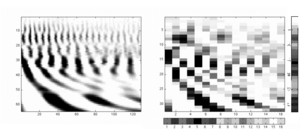
Figure 101 --- Downsampling and marginal calculations for the SAI blocks. The left-hand image shows the full-resolution rectangle from the SAI. The right-hand image shows the region downsampled to 16 × 32 pixels. The mean values of each of the rows and columns of this image are then calculated. These are the marginals which are used as the dense features.

Given this choice of boxes, dense features are computed from each one in turn. The image inside each box is downsampled to the size of the smallest box. This rescaling causes the larger rectangles to be viewed at a coarser resolution. To further reduce the dimensionality, the marginals of the box are computed by averaging over each of the two dimensions, and these two vectors are concatenated to form the final, dense feature vector. For the standard small box size of 16 × 32 this is a 48 dimensional vector. The use of the marginals of each box reduces the dimensionality into the following sparse-code extraction step, while preserving much of the important information about spectral and temporal structure. Figure 101 shows the effect of performing downsampling and computing marginals for a region of the SAI.

Sparse coding

In the next stage of processing, the low-dimensional dense feature vectors from individual boxes are converted to sparse codes by use of vector quantisation (VQ) (Gersho and Gray, 1992). In the training stage, a 'codebook' is learned over a range of sounds using k-means clustering. Dense feature vectors are computed for a representative sample of the audio (in the case of these experiments, the entire training set was used), and they are then assigned to 'clusters' in the high-dimensional dense feature space. In the baseline case, 256 means were used for the k-means clustering. Once the codebooks are trained, encoding a dense feature vector is simply a matter of assigning it to the closest cluster in the codebook. In this way, the 48-dimensional dense feature vector was encoded as a 256-element vector with all elements being zero except a single one at the position of the chosen codeword. Obviously it is trivial to encode such a vector as a single integer: the index of the nonzero element.

Matching pursuit

In addition to the simple VQ scheme described above, we also used a matching pursuit (MP) based encoding scheme to allow a less sparse, but potentially richer representation to be used (Bergeaud and Mallat, 1995; Mallat and Zhang, 1993). In matching pursuit, the dense feature vector to be encoded is matched to the closest codeword in the codebook, as above. However, the process then continues to encode the `residual', the difference between the codeword and the original input. The residual is calculated and is again matched to the closest codeword. This process continues until either the residual is smaller than some limiting value, or the maximum number of codewords is reached. The resulting feature vector in this case is still sparse, in that most of the elements are still zero, but the nonzero elements have values proportional to the amount of the original signal encoded by that particular codeword.

Sound ranking

Using the process in the above stages, a sparse vector is computed for each of the individual boxes tiling the image. These vectors are then concatenated to yield a higher-dimensional sparse feature vector that summarises the entire SAI. This, along with a representation of the text tags used to annotate the audio file, is the input to the PAMIR learning system.

PAMIR

In order to rank audio documents, we wish to learn a scoring function, $S W (q, a)$ , that scores every pair of audio document, $a$ , and query, $q$ . PAMIR (Grangier and Bengio, 2008) uses a bilinear score $S W (q, a) = q T W a$ . The PAMIR system is based on the passive-aggressive family of learning algorithms (Crammer et al., 2006).

The matrix $W$ can be viewed as a linear mapping from audio features to query words. Namely, the product $W a$ is viewed as a `bag of words' description of the audio document, and the dot product of this bag of words with the query words $q$ gives the score.

The scoring function, $q T W a$ , is extremely efficient to compute when $q$ and $a$ are sparse, because the matrix multiplication only requires $O ( | q | | a | )$ operations where $| q |$ and $| a |$ are the number of non-zero values in $q$ and $a$ respectively.

The learning goal is then to learn this matrix $W$ , so that the scoring function gives relevant documents a higher score than irrelevant ones.

$S_W(q_i, a_i^+) > S_W(q_i,a_i^-) + 1 \forall \quad \{q_i, a_i^+, a_i^-\}$

where $a_i^+$ is a document relevant to the query and $a_i^-$ is a document not relevant to the query.

To solve this, a loss function $L W$ is defined.

$L_W = \sum_{(q_i, a_i^+, a_i^-)} l_W(q_i, a_i^+, a_i^-)$

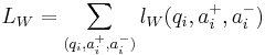
where

$l_W(q_i, a_i^+, a_i^-) = \max\left(0, 1 - S_W(q_i, a_i^+) + S_W(q_i, a_i^-)\right)$

This is a `hinge' loss function. The loss is only nonzero when the system makes a mistake, and so updates to the matrix $W$ only occur at that time.

So $W 0$ is initialised to $0$ , and then at each iteration of the algorithm, a random triplet of $(q_i, a_i^+, a_i^-)$ is picked and $W$ is updated according to the following convex optimisation problem:

$W^i = \mathrm{argmin}_W \frac{1}{2} ||W - W^{i-1}||^2_\mathrm{Fro} + C l_W(q_i, a_i^+, a_i^-)$

Where $| | . | | Fro$ is the Frobenius norm (entry-wise $l 2$ norm on the matrix). At each iteration $i$ , optimising $W i$ achieves a trade-off between remaining close to the previous parameters $W i - 1$ and minimising the loss on the current triplet 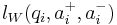$l_W(q_i,a_i^+, a_i^-)$ . The aggressiveness parameter $C$ controls this trade-off.

Experiments

Dataset

The dataset used for the training and testing of the system consisted of 8,638 sound effects, from various sources. 3,855 of these were from commercial sound effects libraries, and the rest from a range of websites<ref>FindSounds, Partners in Rhyme, Acoustica, I Love WAVs, SimplyTheBest Sounds, wav-sounds.com, wavsource.com, and wavlist.com</ref>. Where sounds had text descriptions provided, these were used as a basis for the tagging. Where there was no text description provided, the sounds were listened to and tagged manually with a few key words. Higher-level tags were also added to each file automatically, so for example a file labelled 'cat' would have the tags 'mammal' and 'feliformia' added. Adding these higher-level terms provided some structure to the label space. The text terms were then stemmed using the Porter stemmer for English (Porter, 1980), leaving a total of 3,268 unique tags. The sounds had an average of 3.2 tags each.

Experimental setup

Cross-validation was used to estimate performance of the learned ranking system. Specifically, the set of audio documents was split in three equal parts, using two thirds for training and the remaining third for testing. Training and testing were repeated for all three splits of the data, in order to obtain an estimate of the performance on all the documents. Queries that had fewer than 5 documents in either the training set or the test set were removed from both sets, and the corresponding documents were removed if these contained no other tag. A second level of cross validation was used to determine the values of the aggressiveness parameter C, and the number of training iterations. In general performance was good as long as C was not too high, and lower C values required longer training. A value of C = 0.1 was selected, which was also found to work well in other applications (Grangier and Bengio, 2008), and 10 million iterations. In preliminary experiments, we found that the system was not very sensitive to the value of these parameters. The precision (fraction of positives) within the top k audio documents from the test set as ranked for each query was used to evaluate the quality of the ranking obtained by the learned model.

Auditory features parameters

The process of transformation of SAI frames into sparse codes has several parameters that can be varied. We defined a default parameter set and then performed experiments in which one or a few parameters were varied from this default set.

The default parameters used the Lyon-SAI, cut into rectangles starting with the smallest size of 16 lags by 32 channels, leading to a total of 49 rectangles. All the rectangles were reduced to 48 marginal values each, and for each box a codebook of size 256 was used, leading to a total of 49 × 256 = 12,544 feature dimensions.

From this default experiment, variations were made by systematic modification of the smallest rectangle size used for sparse segmentation and by limiting the maximum number of rectangles used for the sparse segmentation (with variations favouring smaller rectangles and larger rectangles). Further variants used systematic variation of the codebook sizes used in sparse coding (using both standard vector quantisation and matching pursuit). In addition, the AIM-SAI representation was used with otherwise default parameters. The values of all the experimental parameters used are shown in <tablenameRef name="sai_exp_params"/>.

In one group of experiments we varied the details of the box-cutting step. In our baseline we use rectangles of size 16 × 32 and larger, each dimension being multiplied by powers of two, up to the largest size that fits in an SAI frame. We varied the base size of the rectangle, starting from the sizes 8 × 16 and 32 × 64. We also restricted the number of sizes, by limiting the doublings of each dimension. This restriction serves to exclude the global features that are taken across a large part of the auditory image frame. In a separate series of experiments we instead started from a rectangle size equal to the dimensions of the SAI frame, working downwards by repeatedly cutting the horizontal and vertical dimensions in half. This set excludes features that are very local in the auditory image. While the codebook sizes remained fixed at 256, the total number of feature dimensions varied, proportional to the number of boxes used, and performance within each series was found to be monotonic with the total number of feature dimensions.

<tablename name="sai_exp_params"/> Parameters used for the SAI experiments
Parameter Set	Smallest Box	Total Boxes	Means Per Box	VQ	Box Cutting
Default	32x16	49	256	VQ	Up
Codebook Sizes	32x16	49	4, 16, 64, 256, 512, 1024, 2048, 3000, 4096, 6000	VQ	Up
Matching Pursuit	32x16	49	4, 16, 64, 256, 1024, 2048, 3000	MP	Up
Box Sizes (Down)	16x8 32x16 64x32	1, 8, 33, 44, 66 8,12,20,24 1,2,3,4,5,6	256	VQ	Down
Box Sizes (Up)	16x8 32x16 64x32	32, 54, 72, 90, 108 5, 14, 28, 35, 42 2, 4, 6, 10, 12	256	VQ	Up
AIM-SAI	32x16	42	256	VQ	Up

Comparisons with MFCC

For comparison with the auditory features, standard MFCCs were calculated and were converted into a sparse code in the same way as for the dense SAI features. MFCCs were computed using a Hamming window, with the first and second derivatives as additional features of each frame. The initial MFCC parameters were chosen based on a configuration that was optimised for speech, and then three of the parameters were systematically varied: the number of cepstral coefficients (traditionally 13 for speech), the length of each frame (traditionally 25ms) and the number of codebooks used to sparsify the MFCC of each frame. Optimal performance was obtained with a codebook of size 5000, 40ms frames and 40 cepstral coefficients. This configuration corresponds to much higher frequency resolution than the standard MFCC features used for speech.

Results

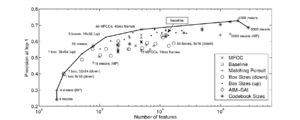
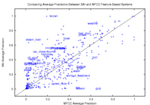
Figure 102 – Precision at top-ranked result as a function of sparse feature vector size. The convex hull joining the extremal points is shown to illustrate the maximal precision for a given feature vector size. The different symbols highlight the experiment sets varying different parameters. Parameters for some experiments are shown on the plot.

Figure 103 – Comparison of average precision for the SAI and MFCC features across various query terms. The crosses are individual query terms, with some marked. The plot is slightly skewed to higher precision for the SAI, but there is no consistent bias to be seen in the types of query terms that are better represented by MFCC or SAI features.

The various parameters of SAI and MFCC feature extraction were varied as shown in <tablenameRef name="sai_exp_params"/>. Figure 102 shows the average precision of the top-ranked result against the length of the sparse feature vector. In each set of experiments, the series of markers show the effect of changing the variable in question. In each experimental case, all other parameters were left at their `baseline' values. Each set of experiments is identified by a different marker. As the number of features becomes very large, performance begins to saturate. The top performance is for the system with 73% at the top-ranked sound file, achieved with 4,000 codewords per codebook and a total of 49 codebooks. This was significantly better than the best MFCC result, which achieved 67% (Wilcoxon test for equal medians, p = 0.0078). This reflects about 18% smaller error (from 33% to 27% error). SAI features also achieve better precision-at-top-k consistently for all values of k, although with lower relative precision improvement. <tablenameRef name="sai_mfcc_error_reduction"/> shows the improvement in precision at top-k for a number of values of k.

<tablename name="sai_mfcc_error_reduction"/> Error reduction from MFCC to SAI features
top-k	SAI	MFCC	Percent error reduction
1	27	33	18%
2	39	44	12%
5	60	62	4%
10	72	74	3%
20	81	84	4%

It is important to note that the parameters found (and the auditory model architecture in general) are not guaranteed to be optimal, and it is possible that further refinement could further improve the retrieval precision.

Performance for the baseline AIM-SAI features (63.6% for 10,752-dimensional features) was very similar to that for the baseline Lyon-SAI features (64.1% for 12,544-dimensional features).

<tablename name="misclassifications"/> Examples of misclassification. All pairs of true-label and confused labels with total count above seven are listed.
Query	Label	Total Number of Errors
clock-tick	cuckoo	8
door knock	door	8
evil laugh	laugh	7
laugh witch	laugh	7
bell-bicycl	bell	7
bee-insect	insect	7

The system described above works only with exact terms, and so related terms are counted as a misclassification. However, people may use many different terms to describe similar sounds. This means that the measured performance of the system will be lower than the actual performance, since many sounds which would be judged by a human listener to be similar are not regarded as such by the system. <tablenameRef name="misclassifications"/> shows some examples of the terms that most frequently caused confusion in the classification system. For each pair of queries we measure confusion by counting the number of sound files that were ranked within the top-k files for the first query, but not for the second query, even though the second query appeared in the labels for the file. For example, there were 7 sound files that were labelled 'evil laugh' but were not ranked within the top k documents for the query 'evil laugh'. At the same time, these documents were ranked highly for the query 'laugh'. Confused queries are often semantically similar to the sound label, and so the errors made by the ranking systems actually reflect the fact that the sound files have partial or inconsistent labelling. In some cases, such as 'clock-tick' and 'cuckoo', the terms are not immediately related, but it is easy to imagine how these sounds would occur together. This effect demonstrates the power of content-based models to identify examples that sound similar, even if their textual labels are incomplete or simply wrong.

Figure 103 compares the performance of the SAI and MFCC systems. The crosses are individual query terms, with some marked. The plot is slightly skewed to higher precision for the SAI (there are more queries above the line than below it). This plot was generated to test the hypothesis that the MFCC features and SAI features might perform better for one class of queries or another. However, there is no particular bias to be seen in which query terms are better represented by MFCC or SAI features.

Conclusions

We developed a content-based sound ranking system that can learn a match between acoustic features of the sound, and a set of text labels. Two different classes of acoustic features were investigated: MFCCs and features based on the SAI. The best performance was achieved with the SAI-based features, although by extending the time window used by the MFCCs, it was also possible to improve performance above the baseline level. The major difference between the MFCC and SAI representations is that SAIs retain better the fine timing information in the signal, whereas MFCCs better preserve the fine spectral structure (especially when the number of MFCC coefficients is large).

The finding that SAI features can give better performance than MFCCs lends support to the hypothesis that a preprocessor that mimics aspects of the human auditory system can produce an effective representation for a machine hearing system. However, the auditory model that we describe above may not always be optimal, and there is potential for improved performance by better characterising the optimal parameters for specific tasks.

The processing performed to generate SAIs involves multiple nonlinear components, and this could be one reason why the features generated from SAIs are more discriminative than standard MFCC features. It is hard to assess exactly why the test sounds appear to be better represented by the features from the auditory model. One difference between SAI and MFCC representations is that SAIs retain fine timing information, while MFCCs preserve fine spectral structure (when the number of coefficients is large enough). However, further study will be required to ascertain exactly what the key properties of the systems involved in going from a sound to a sparse feature vector are, and how these affect performance.

The system described above currently uses only features from short windows. There is much potential for employing methods that deal with the longer-term temporal structure of sounds. Future work in this area should incorporate more dynamics of the sound over longer times, perhaps representing repeating patterns that contain more temporal context.

Conclusions

In this chapter, a full-scale machine-hearing system was developed and deployed for a real content-based audio analysis task. The goal of the study in this chapter was to demonstrate the potential utility of machine hearing systems for audio analysis, and to present a complete example system.

The study presented in this chapter, along with that in chapter 2, both demonstrate a potential benefit in the use of carefully-constructed auditory features over MFCCs for content-based audio analysis tasks. These are both encouraging findings and both point the way for further research into auditory features. One remaining challenge is to find a feature set which is both constrained enough to retain a set of scale-invariant features, and yet rich enough to allow accurate recognition on more challenging datasets. The task of extending to larger-scale problems will be made easier by some key pieces of technology and integration which were developed in the study detailed here. The open-source AIM-C software allows for fast processing of large databases of audio. Coupled with HTK, and a set of scripts allowing distributed processing, this experimental framework can easily be extended to test new AIM modules and new feature extraction mechanisms. AIM-C also supports the 'box-cutting' algorithms developed in this chapter, and the AIM-C systems have been ported to the open-source Marsyas framework for content-based music audio analysis tasks.

The audio search system developed at Google demonstrates the effectiveness of auditory features, and includes some very significant technological achievements. The use of sparse features allows the system to scale to extremely large training datasets through the use of PAMIR. The 'box-cutting' technique for multi-scale analysis of the auditory image allows the capture of both temporal and spectral fine-structure and larger-scale features, while keeping the data rate to a manageable level. There is much scope for further research on the exact form of the features that are present in the auditory image, and what features of the sounds are enhanced by processing through an auditory model.

Notes

Conclusions

The analysis of audio signals based on their content has typically been founded on signal processing techniques chosen for mathematical and engineering expediency. The short-window Fourier transform in particular has generally been used as the first step in many audio processing tasks. However, in understanding sounds, the human auditory system takes a very different approach, and one which has the benefit of several hundred million years of the force of evolution behind it. In this thesis I have investigated the hypothesis that, in order to build automated systems that understand sounds, we would do well to make use of the many tricks that the auditory system has developed over this time. Over the course of this work, I have investigated aspects of the use of auditory models for the automated analysis of sounds, and have obtained a number of results which suggest that taking inspiration from the auditory system is not only a reasonable thing to do, but also useful and technically feasible.

Scale-shift invariant fatures

The first aspect of the auditory system used for inspiration was its apparent ability to generate a stream of information that is invariant to changes in the scale of the source. The results of Smith and Patterson (2005), Ives et al. (2005), Smith et al. (2007) and van Dinther and Patterson (2006) demonstrate that humans are exceptionally good at recognising sounds which have been scaled both in pitch and vocal tract length (acoustic scale) to well beyond the range that is encountered in everyday life. This observation led to the development of a scale-shift invariant feature, which attempts to encode information about spectral shape in a scale-invariant manner. This work was presented in chapter 2. The feature models the smoothed output of an auditory filterbank with a constrained Gaussian mixture model. The effectiveness of this approach was demonstrated in a simple syllable recognition task, where scale-shift invariant features were compared with standard MFCC features for recognising a set of 185 syllables generated from 57 different simulated speakers. When the recogniser was trained on speakers with very similar vocal tract lengths, recognition performance was high across the whole range of speakers when using the scale-shift invariant features. When using standard MFCCs, performance was high around the training speakers, but degraded rapidly as the simulated vocal tract length of the speakers became either smaller or larger than that of the speakers in the training set. However, when simulated, optimal, vocal tract length normalisation (VTLN) was performed on the spectrum before computing the MFCCs, performance was better than that with the auditory features.

The system was capable of generalising well when trained on speakers with a range of vocal tract lengths and glottal pulse rates. Performance both with the scale-shift invariant features and with the MFCC features increased markedly when the system was trained in this way, and overall recognition accuracy was around 99% with either feature set. When VTLN was performed as well, performance rose to 100% accuracy. This result underlines the known inability of MFCCs to normalise for acoustic scale. It is not, however, a surprising result; the scale-shift invariant features were specifically designed to have these properties and the MFCCs were not. Once VTLN is performed, performance recovers and exceeds that obtained with the scale-shift invariant features. This result is also not surprising. It is also important to note that, with the scale-shift invariant features, only one feature vector is required per utterance. A system with optimal VTLN requires a feature vector to be computed for all candidate warpings of the frequency axis, and the optimal warping has to be identified in a separate recognition step. These processes add complexity which suggests that scale-shift invariant features might prove most useful in speech recognition systems where there is no prior over the likely vocal tract length of the speaker, or where speakers cannot be tracked well over time.

It is clear that the scale-shift invariant features proposed here require further research before becoming a useful alternative to MFCCs, but the experiments also make it clear that scale-shift invariant features warrant further research. The rationale for using Gaussians to fit the speech spectrum came from Zolfaghari et al. (2006), who used a low-dimensional Gaussian mixture model to encode speech by tracking formants and other spectral features. There are alternatives to this approach; Mertins and Rademacher (2005), for example, presented an alternative VTL-independent feature based on the cross-correlation between adjacent frames of the spectrum. Their system relies on the fact that the spectral centroid of an utterance will shift as a function of vocal tract length. Cross-correlating adjacent frames will tend to 'normalise' the spectrum (while blurring it), shifting the spectrum of a frame towards the overall spectral centroid and thus giving a signal which is more resistant to shifts in VTL. In future work, the relative benefits of the two approaches could be compared. A further alternative to the Gaussian mixtures might be to use the Fourier transform, rather than the cosine transform, to generate MFCC-like features in which the phase of the components is allowed to vary, as in the Mellin transform described in chapter 4.

The syllable recognition task in this case is fairly limited, and slightly contrived, since it relies on syllables which have been scaled in VTL to simulate the exact effect which is then corrected for. The next step for these features will be to test them on a larger-scale, real-world speech recognition task. Ideally, the features would be assessed by training on one class of speakers, men for example, and then testing on women and children. The system should also be tested against a full VTLN system, and the time taken to compute the scale-shift invariant features compared to the extra time taken to compute many features and optimise recognition over VTL.

Strobe detection for strobed temporal integration

The scale-shift invariant feature representation used in the experiments in chapter 2 was based on the output of an auditory filterbank. However, no further processing based on functional models of the auditory system was performed on the filterbank output. The remaining work in this thesis was based on the auditory image model of peripheral auditory processing (AIM) (Patterson et al., 1992; Patterson et al., 1995). The processing performed in AIM is based on a process known as strobed temporal integration. The key to this process is to locate 'strobe' points in the signal coming from each frequency band in the output of a cochlear model. These strobe points are used to initiate an autocorrelation-like temporal integration process which stabilizes the incoming signal. The process of strobe detection is key to generating the stabilized auditory image (SAI). The SAI is a representation of audio as it might appear in the early stages of the auditory pathway. It is a two-dimensional image which is stable over time when the incoming sound is perceived as being stable. In chapter 3, various systems of strobe point detection for strobed temporal integration were investigated, and a new system, based on the physical constraints on the response of the auditory filters was developed. This new technique was tested along with other strobe systems in a strobe detection task, and was found to be approximately as effective as the best of the original techniques. The work in chapter 3 makes explicit the assumptions being made about the process of strobed temporal integration, thus placing it on a firmer theoretical basis.

One important question is to determine how important accurate strobe detection is for content-based audio analysis systems. The evidence from chapter 6, where a system based on a naive strobe model showed similar performance to that of a system with optimal strobing (chapter 3), suggests that strobed temporal integration is robust, and there may not be a great deal to be gained by finding the optimal strobe point in each channel on each cycle of the sound. However, there were many other differences between the two systems tested in chapter 6, and so the effect of the strobe systems is difficult to discern amongst all the variables. Nevertheless, the theoretical work in chapter 3 shows why current strobe detection systems work well, and it places the choice of parameters on a firm theoretical footing. The benefit of tightly specifying the strobe detection algorithm may be seen in systems designed to perform source separation by preferentially strobing on one source or another. Irino and Patterson (2006) showed how strobes from one source in a mixture could be located, and that this led to a stabilised auditory image in which the activity of the target souce dominated. This suggests that it might be possible to develop an auditory source separation system by dynamically constraining strobing to a target source.

Features from the stabilised auditory image

The stabilised auditory image is a model for an early-stage representation of the incoming signal in the brain. As such, we would like to use it to extract auditory features for machine hearing. In chapter 4, I presented the first of two studies in which features generated from the SAI were used in this way. To compare the SAI representation of audio with purely spectral-based representations, I took the scale-shift independent features developed in chapter 2 and generated similar features from the spectral profiles of various slices of the size-shape image (SSI) -- a representation derived directly from the SAI. I compared performance of the features from the SSI with the features from the neural activity pattern (NAP), derived from the cochlear output used in chapter 2. Performance on the features was once again compared with that on MFCCs, with and without VTLN. In clean speech, performance on the SSI-based features was reduced a little relative to that with NAP-based features. Since the average spectral energy passed in each filterbank band is the same for the NAP and the SAI, this result suggests that better tuning of the process by which the SSI is created from the SAI, and better tuning of the GMM-based features to the SSI output, is required in order to realise their full potential.

However, the performance of the features on the task of syllable recognition in noise was markedly different. In the original syllable recognition experiments the MFCC features performed reasonably well, and MFCCs with optimal VTLN performed excellently. The task was then changed so that the syallable recogniser was trained on a range of examples with different signal-to-noise-ratios (SNRs), and then tested at each SNR in turn. In this case, performance on the NAP-based features was, overall, slightly worse than performance with the MFCC features with optimal VTLN. However, despite starting from a lower baseline, performance of the various SSI-based features degraded considerably more slowly as the level of interfering noise increased, such that by a SNR of +12dB, the features computed from the first slice of the SSI gave better recognition than all of the other features. This result shows the potential benefit for SSI-based features in noise. The next experimental step will be to decouple the use of the SSI from the use of the GMM to generate scale-shift independent features, and instead generate DCT-based features on a number of different slices of the SSI, and evaluate how they compare with MFCCs on a more complicated speech recognition task such at the TIMIT database.

Compressive auditory filtering

The cochlea performs dynamic level compression based on stimulus level. This dynamic response was not included in the simple gammatone filterbank used in the experiments of chapters 2 and 4. In chapter 5, I studied the performance of two alternative cochlear models both of which perform dynamic level compression. Based on an observation by Nick Clarke, that an auditory model with a compressive PZFC filterbank was able to explain the results of a pitch strength detection experiment better than a gammatone filterbank, I assessed the relative performance of various auditory filterbanks on pitch-strength detection tasks.

The stimuli were high-pass filtered iterated rippled noise (IRN) and high-pass filtered harmonic complexes. Both of these stimuli lack energy at the fundamental, but both produce a good signal in temporal models of pitch perception, such as those based on the stabilised auditory image. The well-established dynamic compressive gammachirp (dcGC) filterbank, developed by Toshio Irino, was compared with the pole-zero filter cascade (PZFC) of Dick Lyon, with regard to their ability to explain the strong pitch produced by these stimuli. The dcGC and PZFC differ significantly in their architecture and design. The dcGC is a parallel filterbank, in which dynamic gain control is obtained by sampling the signal level in a higher-frequency 'level estimation' filter, and dynamically adjusting the gain based on that. By contrast, the PZFC is a cascade of filters, in which the output of a high-frequency band-pass filter is fed through a cascade of filters with successively lower peak frequencies. In this case, automatic gain control (AGC) is achieved by a smoothing network that monitors the output of the filterbank at each stage and propagates activity coming from that stage to control the gain of filters in nearby stages.

In the pitch analysis task, the dcGC filterbank was found to produce the greater pitch strength in its default state. However, it proved possible to modify the parameters of the PZFC and (a) make the automatic gain control network very fast-acting, and (b) skew the processing to propagate compression to lower-frequency channels. These modifications led to the PZFC producing similar results to those obtained with the dcGC.

Like the evaluation of strobing systems, this analysis of the compressive properties of auditory filterbanks was necessarily confined to a more limited problem than evaluation of a full machine hearing system. Nevertheless, the results suggest that compression is required in auditory filterbanks if they are to explain human pitch perception accurately. The PZFC is an extremely efficient filterbank implementation, due to its cascade structure, and performs dynamic level compression efficiently. It also seems that its properties could be matched to those of the more computationally-costly dcGC filterbank. The efficiency and dynamic level compression used in the PZFC make it a good candidate for use in machine hearing systems, and indeed it is the filterbank used in the complete system presented in chapter 6.

The next step in the analysis of compressive auditory filterbanks in machine hearing should be to test the overall performance of a machine hearing system with and without the use of dynamic level compression. Of special interest would be to find out which sounds, if any, particularly benefit from the use of a compressive filterbank in the preprocessor.

Sparse features for sound effects ranking

In the final chapter of this thesis, I presented a study undertaken at Google research into building a complete, machine hearing based, sound effects search system. This system draws together aspects of the previous work in this thesis, and demonstrates a complete content-based audio analysis system in which the features are generated from a stabilised auditory image. Performance with the SAI-based features exceeds that with MFCC-based features, even when the MFCCs are extended to encompass a larger temporal window and higher spectral resolution.

The PZFC was used as the cochlear model in this system; it is an efficient compressive auditory filterbank, and as demonstrated in chapter 5, can be made to behave similarly to the more computationally demanding dcGC filterbank. In the best-performing SAI-based system, the auditory images were generated using the 'Lyon' strobe detection mechanism discussed in chapter 3. This mechanism was, found to be suboptimal for the specific task of accurate, on pulse, strobe detection. Thus, it was somewhat surprising to discover that the AIM-SAI system, which made use of a better strobe finding mechanism, was found to support almost identical performance to the Lyon-SAI with baseline parameters. As discussed above, it seems that the exact choice of strobe mechanism is not of great importance because strobed temporal integration is inherently a robust process. It is difficult to tease apart the aspects of these systems which might lead to small changes in overall performance on an open-ended task such as this. In future work, I intend to assess the use of different strobe systems in a source separation task, in order to fully understand the effect of strobe detection on the generation of stabilised auditory images.

In the Google machine hearing system, the auditory features were extracted from the SAI with 'box-cutting'; that is, the SAI was broken up into overlapping boxes of different scales and the contents of each box contributed independently to the sparse code used to represent the image. The sparse features used in this study are not, inherently, scale shift invariant. Rather, box-cutting followed by sparse coding is intended to make it possible to identify spectro-temporal patterns in different regions of the SAI. In future work, I intend to compute sparse multiscale features for representations derived from the SAI such as the SSI and the Mellin image (Irino and Patterson, 2002).

Future work

The field of machine hearing is a relatively new one, and this thesis covers a range of interests within the field -- from the low-level operation of the auditory filterbank, to the choice of feature representation for a particular audio analysis task. From the studies described here there are, of course, myriad possible research paths which could be investigated. I have demonstrated some key applications of machine hearing systems, highlighting the potential utility of such systems for scale-independent speech recognition and content-based audio search.

I believe that the groundwork has been laid for the development of a 'canonical' baseline system for machine hearing systems. Such a system would likely combine the PZFC, as an efficient compressive auditory filterbank, with the 'local maximum' strobe finding algorithm to generate stabilised auditory images. This SAI could be used as the basis of a number of feature representations, either by warping the time-interval axes of the different filterbank channels independently to generate the SSI, or by direct sampling of the SAI itself. The 'box-cutting' sparse features described in chapter 6 present one future direction for feature representations from the SAI. These have been proven in a large-scale content-based audio analysis task, but there are also many other possibilities for feature representations from the SAI. As shown in chapter 5, the temporal profile of the SAI can provide a pitch track, even for stimuli which lack a strong harmonic structure, and the scale shift invariant features developed in chapter 2 show a potential route for the scale-independent analysis of audio.

Many of the individual components of machine hearing systems are well-understood, but the study of integrated machine hearing systems is still a developing field. There is still much to be done to understand the exact effect that changes to the low-level components of a machine hearing system have on the high-level behaviour of the system, but given a strong baseline system to work from, I hope that this task will become easier. Many of the tools developed in this thesis may prove useful for the future study of machine hearing. The source code for AIM-C is available online under the Apache 2.0 licence which allows for free copying and development for both commercial and noncommercial applications. AIM-C contains modules which can be combined to generate the scale-shift invariant features used in the syllable recognition task, and the AIM-SAI variant of the sparse feature representation described in chapter 6. Furthermore, there are also modules in AIM-C for the generation of the box-cutting features and sparse codes. Many of the AIM-C modules have been ported to the Marsyas framework for music analysis by Steven Ness, and indeed the sparse features from box-cutting were used as the basis for an entry to the 2010 MIREX music genre classification challenge. As such, the AIM-C modules developed here provide an excellent basis for the future study of machine hearing systems. I'm very excited by the future of machine hearing and I look forward to testing the performance of, and putting to work, ever-improving feature representations based on an understanding of human audition.

Bibliography

Aertsen, A. and Johannesma, P. (1980). “Spectro-temporal receptive fields of auditory neurons in the grassfrog. I. Characterization of tonal and natural stimuli.” Biol. Cybern, 38, p.223-234. [1]
Baker, R.J., Rosen, S. and Darling, A.M. (1998). “An efficient characterisation of human auditory filtering across level and frequency that is also physiologically reasonable”, in Psychophysical and Physiological Advances in Hearing, Palmer, A.R., Rees, A., Summerfield, A.Q. and Meddis, R. editors, p.81-87 (Whurr). [1] [2] [3] [4]
Benzeghiba, M., De Mori, R., Deroo, O., Dupont, S., Erbes, T., Jouvet, D., Fissore, L., Laface, P., Mertins, A., Ris, C. and Others (2007). “Automatic speech recognition and speech variability: A review.” Speech Commun., 49, p.763-786. [1]
Bergeaud, F. and Mallat, S.G. (1995). “Processing images and sounds with matching pursuits.” Booktitle : Proceedings of SPIE. Volume : 2569. OriginalCiteRef : bergeaud1995processing. Pages : 2-. [1]
Bergstra, J., Casagrande, N., Erhan, D., Eck, D. and Kégl, B. (2006). “Aggregate features and ADABOOST for music classification.” Machine Learning, 65, p.473-484. [1] [2]
Bilsen, F.A. (2006). “Repetition pitch glide from the step pyramid at Chichen Itza.” J. Acoust. Soc. Am., 120, p.594-. [1]
Bleeck, S., Ives, T. and Patterson, R.D. (2004). “Aim-mat: The Auditory Image Model in MATLAB.” Acta Acustica, 90, p.781-787. [1]
Brandenburg, K. and Stoll, G. (1994). “ISO-MPEG-1 Audio: A generic standard for coding of high-quality digital audio.” Journal of the Audio Engineering Society, 42, p.780-792. [1]
Bridle, J. and Brown, M. (1974). “An experimental automatic word recognition system.” JSRU Report, 1003, p.. [1]
Brown, G.J. and Cooke, M. (1994). “Computational auditory scene analysis.” Computer speech and language, 8, p.297-336. [1]
Carney, L.H., McDuffy, M.J. and Shekhter, I. (1999). “Frequency glides in the impulse responses of auditory-nerve fibers.” J. Acoust. Soc. Am., 105, p.2384-2391. [1]
Cohen, L. (1993). “The scale representation.” IEEE Trans. Sig. Proc., 41, p.3275-3292. [1] [2]
Cooke, M.P. (1993). Modelling auditory processing and organization. (Cambridge University Press). [1]
Crammer, K., Dekel, O., Keshet, J., Shalev-Shwartz, S. and Singer, Y. (2006). “Online passive-aggressive algorithms.” The Journal of Machine Learning Research, 7, p.585-. [1]
Davis, S.B. and Mermelstein, P. (1990). “Comparison of parametric representations for monosyllabic word recognition in continuously spoken sentences.” Readings in speech recognition, , p.65-74. [1]
de Boer, E. (1975). “Synthetic whole-nerve action potentials for the cat.” J. Acoust. Soc. Am., 58, p.1030-. [1]
de Cheveigné, A. and Kawahara, H. (1999). “Missing-data model of vowel identification.” J. Acoust. Soc. Am., 105, p.3497-3508. [1]
Dempster, A.P., Laird, N.M., Rubin, D.B. and Others (1977). “Maximum likelihood from incomplete data via the EM algorithm.” Journal of the Royal Statistical Society. Series B (Methodological), 39, p.1-38. [1]
Dudley, H. (1939). “Remaking speech.” J. Acoust. Soc. Am., 11, p.169-177. [1] [2]
Fant, G. (1960). Acoustic Theory of Speech Production. (Mouton De Gruyter, The Hague). [1]
Feldbauer, C., Monaghan, J.J. and Patterson, R.D. (2008). “Continuous estimation of VTL from vowels using a linearly VTL-covariant speech feature.” J. Acoust. Soc. Am., 123, p.3339. [1]
Fitch, W.T. and Giedd, J. (1999). “Morphology and development of the human vocal tract: A study using magnetic resonance imaging.” J. Acoust. Soc. Am., 106, p.1511-1522. [1]
Flanagan, J.L. and Guttman, N. (1960). “On the pitch of peridic pulses.” J. Acoust. Soc. Am., 32, p.1308-1319. [1]
Fletcher, H. (1940). “Auditory patterns.” Reviews of Modern Physics, 12, p.47-65. [1]
Ganchev, T., Fakotakis, N. and Kokkinakis, G. (2005). “Comparative evaluation of various MFCC implementations on the speaker verification task.” Booktitle : Proceedings of the SPECOM. Volume : 1. Organization : Citeseer. OriginalCiteRef : ganchev2005comparative. Pages : 191-194. [1]
Gersho, A. and Gray, R.M. (1992). “Vector quantization and signal compression..” Publisher : Kluwer Academic Publishers. OriginalCiteRef : gersho-vector. [1]
Glasberg, B.R. and Moore, B.C.J. (2000). “Frequency selectivity as a function of level and frequency measured with uniformly exciting notched noise.” J. Acoust. Soc. Am., 108, p.2318-2328. [1] [2] [3]
Glasberg, B.R. and Moore, B.C.J. (2002). “A model of loudness applicable to time-varying sounds.” Journal of the Audio Engineering Society, 50, p.331-342. [1]
Gomersall, P.A., Walters, T.C. and Patterson, R.D. (2005). “Size and temperature information in bullfrog calls.” Howpublished : Poster, British Society of Audiology short papers meeting, Cardiff, UK. OriginalCiteRef : gomersall:2005. [1]
Grangier, D. and Bengio, S. (2008). “A discriminative kernel-based model to rank images from text queries.” IEEE Trans. Pattern Anal. Mach. Intell., , p.1371-1384. [1] [2] [3]
Gray, H. (1918). Anatomy of the human body. (Lea \& Febiger). [1]
Greenberg, S. and Ainsworth, W.A. (2006). Listening to speech: an auditory perspective. (Lawrence Erlbaum). [1]
Handel, S. and Patterson, R.D. (2000). “The perceptual tone/noise ratio of merged, iterated rippled noises with octave, harmonic, and nonharmonic delay ratios.” J. Acoust. Soc. Am., 108, p.692-695. [1]
Hawks, J.W. and Miller, J.D. (1995). “A formant bandwidth estimation procedure for vowel synthesis.” J. Acoust. Soc. Am., 97, p.1343-1345. [1] [2]
Hess, W. (1983). Pitch determination of speech signals: algorithms and devices. (Springer-Verlag). [1] [2] [3] [4] [5] [6]
Huang, X., Acero, A. and Hon, H.W. (2001). Spoken language processing: A guide to theory, algorithm, and system development. (Prentice Hall PTR Upper Saddle River, NJ, USA). [1]
Huber, J.E., Stathopoulos, E.T., Curione, G.M., Ash, T.A. and Johnson, K. (1999). “Formants of children, women, and men: The effects of vocal intensity variation.” J. Acoust. Soc. Am., 106, p.1532-1542. [1] [2]
Huygens, C. (1693). “En envoiant le probleme d'Alhazen en France.” Date-added : 2009-11-27 16:56:45 +0000. Date-modified : 2009-11-27 16:58:28 +0000. Howpublished : printed in Oeuvres Compl{\`e}tes, Vol. 10, edited by Societ{\'y} Hollandaise des Sciences (Nijhoff, Den Haag, 1950), pp.570--571. OriginalCiteRef : huygens:1693. [1]
Irino, T., Patterson, R.D. and Kawahara, H. (2006). “Speech segregation using an auditory vocoder with event-synchronous enhancements.” IEEE Trans. Audio, Speech, and Language Process., 14, p.2212-2221. [1]
Irino, T., Walters, T.C. and Patterson, R.D. (2007). “A computational auditory model with a nonlinear cochlea and acoustic scale normalization”, in Proceedings of the 19th International Congress on Acoustics, p.07-003. [1]
Irino, T. and Patterson, R.D. (1997). “A time-domain, level-dependent auditory filter: The gammachirp.” J. Acoust. Soc. Am., 101, p.412-419. [1] [2] [3]
Irino, T. and Patterson, R.D. (2001). “A compressive gammachirp auditory filter for both physiological and psychophysical data.” J. Acoust. Soc. Am., 109, p.2008-2022. [1]
Irino, T. and Patterson, R.D. (2002). “Segregating Information about the Size and Shape of the Vocal Tract using a Time-Domain Auditory Model: The Stabilised Wavelet-Mellin Transform.” Speech Commun., 36, p.181-203. [1] [2] [3]
Irino, T. and Patterson, R.D. (2006). “A Dynamic Compressive Gammachirp Auditory Filterbank.” IEEE Transactions on Audio, Speech, and Language Processing, 14, p.2222-2232. [1] [2] [3] [4] [5] [6] [7]
Irino, T. and Unoki, M. (1999). “An analysis/synthesis auditory filterbank based on an IIR implementation of the gammachirp.” J. Acoust. Soc. Jpn, 20, p.397-406. [1]
Ives, D.T., Smith, D.R.R. and Patterson, R.D. (2005). “Discrimination of speaker size from syllable phrases.” J. Acoust. Soc. Am., 118, p.3816-3822. [1] [2] [3] [4] [5]
Ives, D.T. and Patterson, R.D. (2008). “Pitch strength decreases as F0 and harmonic resolution increase in complex tones composed exclusively of high harmonics.” J. Acoust. Soc. Am., 123, p.2670-9. [1] [2] [3] [4] [5] [6]
Johannesma, P. (1972). “The pre-response stimulus ensemble of neurons in the cochlear nucleus.” Pages : 58-69. Booktitle : IPO Symposium on Hearing Theory. IPO, Eindhoven, The Netherlands. OriginalCiteRef : johannesma1972pre. [1]
Kawahara, H., Masuda-Katsuse, I. and de Cheveigné, A. (1999). “Restructuring speech representations using a pitch-adaptive time-frequency smoothing and an instantaneous-frequency-based F0 extraction: Possible role of a repetitive structure in sounds.” Speech Comm., 27, p.187-207. [1] [2]
Kawahara, H. and Irino, T. (2004). “Underlying principles of a high-quality speech manipulation system STRAIGHT and its application to speech segregation”, in Speech separation by humans and machines, Divenyi, P.L. editor, p.167-180 (Kluwer Academic). [1] [2]
Kim, D.O., Molnar, C.E. and Matthews, J.W. (1980). “Cochlear mechanics: nonlinear behaviour in two-tone responses as reflected in cochlear-nerve-fibre responses and in ear-canal sound pressure.” J. Acoust. Soc. Am., 67, p.1704-1721. [1]
Krumbholz, K., Patterson, R.D., Nobbe, A. and Fastl, H. (2003). “Microsecond temporal resolution in monaural hearing without spectral cues?.” J. Acoust. Soc. Am., 113, p.2790-2800. [1]
Krumbholz, K., Patterson, R.D. and Pressnitzer, D. (2000). “The lower limit of pitch as determined by rate discrimination.” J. Acoust. Soc. Am., 108, p.1170-1180. [1]
Ladefoged, P. and Broadbent, D.E. (1957). “Information Conveyed by Vowels.” J. Acoust. Soc. Am., 29, p.98-104. [1]
Lee, S., Potamianos, A. and Narayanan, S. (1999). “Acoustics of children's speech: developmental changes of temporal and spectral parameters.” J. Acoust. Soc. Am., 105, p.1455-68. [1]
Lutfi, R.A. and Patterson, R.D. (1984). “On the growth of masking asymmetry with stimulus intensity.” J. Acoust. Soc. Am., 76, p.739-745. [1]
Lyon, R.F. (1996). “The All-Pole Gammatone Filter and Auditory Models.” Journal : unpublished. OriginalCiteRef : Ldraft96. Uri : http://dicklyon.com/tech/Hearing/APGF_Lyon_1996.pdf. [1]
Lyon, R.F. (1997). “All-pole models of auditory filtering”, in Diversity in Auditory Mechanics, E. R. Lewis, S.C. and Lyon, R.F. editors, p.205-211 (World Scientific Publishing, Singapore). [1]
Lyon, R.F. (1998). “Filter cascades as analogs of the cochlea.” Hum. Mov. Sci., , p.3-18. [1] [2] [3] [4]
Lyon, R.F., Katsiamis, A.G. and Drakakis, E.M. (2010). “History and Future of Auditory Filter Models.” OriginalCiteRef : . Booktitle : IEEE International Symposium on Circuits and Systems, 2010. ISCAS 2007. [1] [2] [3] [4] [5]
Lyon, R.F., Rehn, M., Bengio, S., Walters, T.C. and Chechik, G. (2010). “Sound retrieval and ranking using auditory sparse- code representations.” Journal : Neural Computation. Note : Under review. OriginalCiteRef : lyon:2010a. [1]
Lyon, R.F. and Mead, C. (1988). “An analog electronic cochlea.” IEEE Transactions on Acoustics Speech and Signal Processing, 36, p.1119-1134. [1] [2]
Mallat, S.G. and Zhang, Z. (1993). “Matching pursuits with time-frequency dictionaries.” IEEE Transactions on Signal Processing, 41, p.3397-3415. [1]
Mermelstein, P. (1976). “Distance measures for speech recognition, psychological and instrumental.” Pattern Recognition and Artificial Intelligence, , p.374-388. [1]
Mertins, A. and Rademacher, J. (2005). “Vocal tract length invariant features for automatic speech recognition.” Booktitle : 2005 IEEE Workshop on Automatic Speech Recognition and Understanding. OriginalCiteRef : mertins2005vocal. Pages : 308-312. [1] [2] [3]
Miller, G.A. and Licklider, J.C.R. (1950). “The intelligibility of interrupted speech.” J. Acoust. Soc. Am., 22, p.167-173. [1]
Monaghan, J.J., Feldbauer, C., Walters, T.C. and Patterson, R.D. (2008). “Low-dimensional, auditory feature vectors that improve vocal-tract-length normalization in automatic speech recognition.” J. Acoust. Soc. Am., 123, p.3066. [1] [2]
Moore, B.C.J. (1995). Hearing. (Academic Press). [1]
Moore, B.C.J. (2003). An Introduction to the Psychology of Hearing. (Academic Press). [1] [2] [3] [4]
Moore, B.C.J., Peters, R.W. and Glasberg, B.R. (1990). “Auditory filter shapes at low center frequencies.” J. Acoust. Soc. Am., 88, p.132-140. [1]
Olshausen, B.A. and Field, D.J. (2004). “Sparse coding of sensory inputs.” Curr. Opin. Neurobiol., 14, p.481-487. [1]
Patterson, R., Holdsworth, J., Nimmo-Smith, I. and Rice, P. (1988). “SVOS final report: The auditory filterbank.” APU report, 2341, p.. [1]
Patterson, R.D. (1994). “The sound of a sinusoid: Spectral models.” J. Acoust. Soc. Am., 96, p.1409-1418. [1] [2]
Patterson, R.D. (1994). “The sound of a sinusoid: Time-interval models.” J. Acoust. Soc. Am., 96, p.1419-1428. [1] [2] [3]
Patterson, R.D., Allerhand, M.H. and Giguère, C. (1995). “Time-domain modeling of peripheral auditory processing: A modular architecture and a software platform.” J. Acoust. Soc. Am., 98, p.1890-1894. [1] [2] [3] [4] [5]
Patterson, R.D., Handel, S., Yost, W.A. and Datta, A.J. (1996). “The relative strength of the tone and noise components in iterated rippled noise.” J. Acoust. Soc. Am., 100, p.3286-3294. [1] [2] [3] [4] [5] [6] [7] [8] [9]
Patterson, R.D., Nimmo-Smith, I., Weber, D.L. and Milroy, R. (1982). “The deterioration of hearing with age: frequency selectivity, the critical ratio, the audiogram, and speech threshold.” J. Acoust. Soc. Am., 72, p.1788-1803. [1]
Patterson, R.D., Robinson, K., Holdsworth, J., McKeown, D., Zhang, C. and Allerhand, M. (1992). “Complex Sounds and Auditory Images”, in Auditory Physiology and Perception, Y Cazals L. Demany and Horner, K. editors (Pergamon Press, Oxford). [1] [2] [3] [4]
Patterson, R.D., Smith, D.R.R., van Dinther, R. and Walters, T.C. (2008). “Size Information in the Production and Perception of Communication Sounds”, in Auditory Perception of Sound Sources, Yost, W.A., Popper, A.N. and Fay, R.R. editors (Springer Science+Business Media, LLC, New York). [1] [2]
Patterson, R.D., Unoki, M. and Irino, T. (2003). “Extending the domain of center frequencies for the compressive gammachirp auditory filter.” J. Acoust. Soc. Am., 114, p.1529-1542. [1] [2] [3] [4] [5] [6] [7] [8] [9]
Patterson, R.D., van Dinther, R. and Irino, T. (2007). “The robustness of bio-acoustic communication and the role of normalization”, in Proceedings of the 19th International Congress on Acoustics, p.07-011. [1] [2]
Patterson, R.D., Walters, T.C., Monaghan, J., Feldbauer, C. and Irino, T. (2010). “Auditory speech processing for scale-shift covariance and its evaluation in automatic speech recognition.” Booktitle : IEEE International Symposium on Circuits and Systems, 2010. ISCAS 2010. Notes : submitted. OriginalCiteRef : . [1]
Patterson, R.D., Yost, W.A., Handel, S. and Datta, A.J. (2000). “The perceptual tone/noise ratio of merged iterated rippled noises.” J. Acoust. Soc. Am., 107, p.1578-1588. [1]
Patterson, R.D. and Irino, T. (1998). “Modeling temporal asymmetry in the auditory system.” J. Acoust. Soc. Am., 104, p.2967-2979. [1]
Patterson, R.D. and Moore, B.C.J. (1986). “Auditory filters and excitation patterns as representations of frequency resolution”, in Frequency Selectivity in Hearing, Moore, B.C. editor (Academic Press, London). [1]
Peterson, G.E. and Barney, H.L. (1952). “Control Methods Used in a Study of the Vowels.” J. Acoust. Soc. Am., 24, p.175-184. [1] [2]
Porter, M. (1980). “An algorithm for suffix stripping.” Program, 14, p.130-137. [1]
Purgue, A. (1997). “Tympanic sound radiation in the bullfrog Rana catesbeiana.” Journal of Comparative Physiology A: Neuroethology, Sensory, Neural, and Behavioral Physiology, 181, p.438-445. [1]
Rehn, M., Lyon, R.F., Bengio, S., Walters, T.C. and Chechik, G. (2009). “Sound Ranking Using Auditory Sparse-Code Representations”, in International Conference on Machine Learning 2009, Workshop: Sparse Methods for Music Audio, Montr{\'e}al, Canada. [1]
Rhode, W.S. and Cooper, N.P. (1993). “Two-tone suppression and distortion production on the basilar membrane in the hook region of the cat and guinea pig cochleae.” Hear. Res., 66, p.31-45. [1]
Rhode, W.S. and Robles, L. (1974). “Evidence from Mössbauer experiments for non-linear vibration in the cochlea.” J. Acoust. Soc. Am., 55, p.588-596. [1]
Robinson, K. and Patterson, R.D. (1995). “The stimulus duration required to identify vowels, their octave and their timbre.” J. Acoust. Soc. Am., 98, p.1858-1865. [1]
Rosen, S. and Baker, R.J. (1994). “Characterising auditory filter nonlinearity.” Hear. Res., 73, p.231-243. [1]
Ruggero, M.A., Robles, L. and Rich, N.C. (1992). “Two-tone suppression in the basilar membrane of the cochlea: Mechanical basis of auditory-nerve rate suppression.” J. Neurophysiol., 68, p.1087-1099. [1]
Sachs, M.B. and Kiang, N.Y.S. (1968). “Two-tone inhibition in auditory nerve fibers.” J. Acoust. Soc. Am., 43, p.1120-1128. [1]
Schofield, D. (1985). “Visualisations of speech based on a model of the peripheral auditory system.” Unknown, , p.. [1]
Schreiner, C.E. and Langner, G. (1988). “Periodicity coding in the inferior colliculus of the cat. II. Topographical organization.” J. Neurophysiol., 60, p.1823-. [1]
Slaney, M. (1993). An Efficient Implementation of the Patterson-Holdsworth Auditory Filter Bank Apple technical Report. [1] [2]
Slaney, M. (1993). “Auditory toolbox.” Apple Computer Company: Apple Technical Report, 45, p.. [1]
Slaney, M., Naar, D. and Lyon, R.F. (1994). “Auditory model inversion for sound separation.” Booktitle : Proceedings of 1994 International Conference on Acoustics, Speech, and Signal Processing. Volume : 2. Organization : Citeseer. OriginalCiteRef : slaney1994auditory. Pages : 77-80. [1]
Smith, D.R.R., Patterson, R.D., Turner, R.E., Kawahara, H. and Irino, T. (2005). “The processing and perception of size information in speech sounds.” J. Acoust. Soc. Am., 117, p.305-318. [1] [2] [3] [4] [5] [6]
Smith, D.R.R., Walters, T.C. and Patterson, R.D. (2007). “Discrimination of speaker sex and size when glottal-pulse rate and vocal-tract length are controlled.” J. Acoust. Soc. Am., 122, p.3628-3639. [1] [2] [3] [4]
Smith, D.R.R. and Patterson, R.D. (2005). “The interaction of glottal-pulse rate and vocal-tract length in judgements of speaker size, sex, and age.” J. Acoust. Soc. Am., 118, p.3177-3186. [1] [2] [3]
Smith, J.O. and Abel, J.S. (1999). “Bark and ERB bilinear transforms.” IEEE Transactions on Speech and Audio Processing, 7, p.697-708. [1]
Sprague, M.W. (2000). “The single sonic muscle twitch model for the sound-production mechanism in the weakfish, Cynoscion regalis.” J. Acoust. Soc. Am., 108, p.2430-2437. [1]
Stevens, S., Volkmann, J. and Newman, E. (1937). “A scale for the measurement of the psychological magnitude pitch.” J. Acoust. Soc. Am., 8, p.185-. [1]
Stuttle, M. and Gales, M. (2001). “A mixture of Gaussians front end for speech recognition.” Booktitle : Seventh European Conference on Speech Communication and Technology. Organization : Citeseer. OriginalCiteRef : stuttle2001mixture. [1]
Turner, R.E., Walters, T.C., Monaghan, J.J. and Patterson, R.D. (2009). “A statistical, formant-pattern model for segregating vowel type and vocal-tract length in developmental formant data.” J. Acoust. Soc. Am., 125, p.2374-2386. [1] [2] [3] [4] [5] [6]
Turner, R.E., Walters, T.C. and Patterson, R.D. (2004). “Estimating vocal tract length from formant frequency data using a physical model and a latent variable factor analysis”, in British Society of Audiology Short Papers Meeting on Experimental Studies of Hearing and Deafness, p.61-. [1]
Turner, R.E. and Patterson, R.D. (2003). “An analysis of the size information in classical formant data: Peterson and Barney (1952) revisited.” Journal of the Acoustical Society of Japan, 33, p.585-589. [1]
Unoki, M., Irino, T., Glasberg, B., Moore, B.C. and Patterson, R.D. (2006). “Comparison of the roex and gammachirp filters as representations of the auditory filter.” J. Acoust. Soc. Am., 120, p.1474-1492. [1] [2]
Unoki, M., Irino, T. and Patterson, R.D. (2001). “Improvement of an IIR asymmetric compensation gammachirp filter.” Acoustical Science and Technology, 22, p.426-430. [1] [2] [3]
van Dinther, R. and Patterson, R.D. (2006). “Perception of acoustic scale and size in musical instrument sounds.” J. Acoust. Soc. Am., 120, p.2158-76. [1] [2] [3]
Vestergaard, M.D., Fyson, N.R.C. and Patterson, R.D. (2009). “The interaction of vocal tract length and glottal pulse rate in the recognition of concurrent syllables.” J. Acoust. Soc. Am., 125, p.1114-1124. [1]
von Békésy, G. (1960). Experiments in Hearing. (McGraw-Hill). [1]
von Helmholtz, H.L.F. (1875). On the Sensations of Tone as a Physiological Basis for the Theory of Music. (Longmans, Green and Co.). [1]
Walters, T.C., Gomersall, P.A., Turner, R.E. and Patterson, R.D. (2008). “Comparison of relative and absolute judgments of speaker size based on vowel sounds.” Proceedings of Meetings on Acoustics, 1, p.1-9. [1] [2]
Welling, L., Ney, H. and Kanthak, S. (2002). “Speaker adaptive modeling by vocal tract normalization.” IEEE Transactions on Speech and Audio Processing, 10, p.415-426. [1] [2] [3] [4]
Wever, E.G. (1949). Theory of hearing. (Wiley). [1]
Yost, W.A. (1996). “Pitch of iterated rippled noise.” J. Acoust. Soc. Am., 100, p.511-518. [1]
Yost, W.A., Patterson, R. and Sheft, S. (1996). “A time domain description for the pitch strength of iterated rippled noise.” J. Acoust. Soc. Am., 99, p.1066-1078. [1] [2]
Yost, W.A., Patterson, R. and Sheft, S. (1998). “The role of the envelope in processing iterated rippled noise.” J. Acoust. Soc. Am., 104, p.2349-2361. [1] [2] [3]
Yost, W.A. and Hill, R. (1979). “Models of the pitch and pitch strength of ripple noise.” J. Acoust. Soc. Am., 66, p.400-. [1]
Young, S., Evermann, G., Gales, M., Hain, T., Kershaw, D., Moore, G., Odell, J., Ollason, D., Povey, D., Valtchev, V. and Woodland, P. (2005). The HTK Book. (Microsoft and Cambridge University engineering Department (download from http://htk.eng.cam.ac.uk/)). [1] [2] [3]
Zolfaghari, P., Kato, H., Minami, Y., Nakamura, A., Katagiri, S. and Patterson, R. (2006). “Dynamic Assignment of Gaussian Components in Modelling Speech Spectra.” The Journal of VLSI Signal Processing, 45, p.7-19. [1] [2]
Zweig, G., Lipes, R. and Pierce, J. (1976). “The cochlear compromise.” J. Acoust. Soc. Am., 59, p.975-. [1]

Auditory-Based Processing of Communication Sounds

From CNBH Acoustic Scale Wiki

Contents

Introduction

Communication sounds

Size information in communication sounds

The scaling of communication sounds

Human perception of size

The auditory image model

The human auditory system

Example stimuli

Outer and middle ear

The cochlea

Neural activity pattern

Strobed temporal integration

Software

Invariance properties of the auditory system

Time-frequency and time-scale uncertainty relations

MFCCs

This thesis

Footnotes

Scale-shift Invariant Auditory Features

Introduction

Size information in MFCCs

Scale-shift invariant representations

Features for size-independent speech recognition

Introduction

Scaled syllables

Scale-shift invariant features

Expectation maximisation for Gaussian fitting

Calculating spectral profiles

Feature vectors

HTK for syllable recognition

Experiments

Results

Tuning HMM parameters

Feature comparison

Comparison with standard VTLN

Comparison of computational complexity

Comparison with wide-range training

Conclusions

Strobes and Stabilised Auditory Images

Strobe finding in AIM

Relationship to pitch detection

Thresholding

Windowing

Look-ahead

Noises and damped/ramped sounds

Cross-channel constraints

A set of criteria for good strobe detection

Choosing the correct threshold

Filterbank and vocal tract impulse responses

Single-pulse excitation

Pulse-resonance excitation

Adding a carrier

Multiple pulses

Noise excitation

The effect of low-pass filtering and compression

A candidate system: Low-latency thresholding with constraints

Time constants in each channel

A candidate system: Event-time back-projection

Testing strobe detection

Test stimuli

Methods

Results

Single-source stimuli

Multi-source stimuli

Discussion

Conclusions

Features from the Auditory Image

The stabilised auditory image

SAI marginals

Undersampling

The SSI

The form of the information in the SSI

Dimensionality reduction

Profiles and slices of the size-shape image

Experiments

Comparison with features from the NAP

Testing in noise