Auditory-Based Processing of Communication Sounds/Strobes and Stabilised Auditory Images
From CNBH Acoustic Scale Wiki
Thomas C. Walters
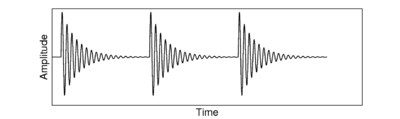
The last chapter introduced a feature representation based on the smoothed output from a simulation of the cochlea and a simple hair-cell model. The signal was temporally averaged over a short window by means of a low-pass filter. Strobed temporal integration, leading to a stabilised auditory image (SAI), is an alternative, more complex, system for processing the signal leaving the cochlea. Strobe points are identified in each channel of the filterbank output, and these points act as triggers for a temporal integration process in which shifted copies of the signal are overlaid on one another.
Since strobe points tend to occur at or near the pulses in a pulse-resonance sound, representing a signal containing a pulse-resonance sound as an SAI will tend to accentuate the periodic, pulse-resonance components of a signal relative to any background noise. Noise-robustness is an extremely useful property in any machine hearing system, and so we wanted to incorporate the inherent noise-robustness of the SAI into our auditory model. In this chapter, existing mechanisms for strobed temporal integration are assessed and compared, and the theoretical basis of this mode of temporal integration is investigated in an effort to identify a simple criterion for optimal strobe generation. The goal was to create a stabilised auditory image for a noise-robust machine hearing system.
Contents |
Strobe finding in AIM
In the auditory image model, stabilised auditory images are produced by strobed temporal integration. An image is built up by repeatedly adding sections of a NAP signal to a buffer. Each time a `significant' event or `strobe' occurs in the signal, the process restarts, adding the signal following the strobe to the buffer, starting at zero. Strobed temporal integration is central to the production of SAIs.
When processing a pulse-resonance communication sound in AIM, it is desirable that the strobe points should fall at points in the NAP signal which were caused by a pulse in the original sound. When this occurs, the resonances following each pulse are added exactly in phase in the auditory image, such that the resonances following each vertical ridge in the image resemble as closely as possible the original resonances in the sound. However, this requirement is somewhat ambiguous because the response of the auditory filterbank to a pulse is not a single peak, but a series of peaks within an envelope.
In practice, it is not necessary for the strobe finding to be perfectly accurate in order that a good SAI be built up from a pulse-resonance sound. The exact choice of which peak of the filter's impulse response to strobe on does not make a significant difference to the auditory image that is produced, and there does not have to be exactly one strobe for each glottal cycle. However, the closer that it is possible to get these requirements, the more accurate the SAI will be. It is desirable that there should be roughly one strobe per pulse, that the choice of strobe points should be reasonably consistent across channels and across pulses and that strobe timing should not be affected too greatly by the exact form of the resonance following each pulse.
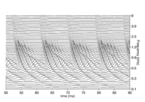
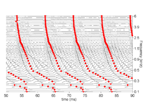
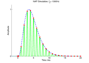
Figure 1 shows the neural activity pattern (NAP) from a short segment of an /a/ vowel. Figure 2 shows a set of strobe points on that NAP. There is exactly one strobe point per cycle in each channel, and the strobe points occur consistently at the peak of the envelope in each channel, so in some sense the algorithm applied here has found the optimal set of strobe points for this signal.
Relationship to pitch detection
Strobe-point detection is, in some respects, a similar process to pitch determination of a time-domain signal (albeit a signal which may have been passed through a nonlinear filter). Computational auditory models which can extract the pitch of complex sounds (see, for example, Brown and Cooke, 1994) must, necessarily, integrate over a few cycles of the pitch period to get a result. Robinson and Patterson (1995) showed that humans take between four and eight cycles of the waveform to extract useful pitch information, but the information required to identify a vowel can be extracted from a single cycle of the wave, and so it is unlikely that long-term pitch extraction can play a direct role in timbre extraction. However, the task of instantaneous detection of peaks in the time-domain waveform is still related to that of pitch detection in the time domain.
There is a rich literature on the subject of pitch detection in time-domain signals and Hess (1983) provides an excellent overview of the state of the field at that time.
Hess identifies four significant features from which periodicity in a signal can be derived in the time domain. The first two of these features are:
- The presence of a fundamental harmonic.
- A structural pattern which repeats from period to period.
The second pair of features is derived from the linear model of speech production, which is the production mechanism for pulse-resonance communication sounds described in chapter 1. Using this model, Hess identifies the following:
- High amplitudes at the start of a period and low amplitudes at the end, since the vocal tract can be assumed to be a linear passive system whose impulse response consists of exponentially decaying sinusoids (Fant, 1960).
- Discontinuities in the signal or its derivatives at the instants where individual pulses occur.
The pitch determination algorithms reviewed by Hess are, of course, all based on analysis of the original waveform, rather than the output of an auditory filterbank, but the principles in each case are similar, and the temporal features which he describes translate to the filtered case.
The majority of algorithms for strobe finding employed in AIM rely on the third of Hess's features to perform their classification of strobe points. When a pulse excites resonances which decay with a finite time constant, an exponential threshold which decays more slowly than the resonance can be applied to the signal to `follow' the decaying resonances. When this threshold is exceeded, a pulse is deemed to have occurred. This simple idea has been proposed and implemented many times; indeed Hess cites over 20 references to proposals for analogue versions of this scheme dating from 1949 to 1977.
In this section, I review some of the basic properties of the auditory filterbank and human vocalisations to help derive the correct constraints for a strobing scheme that is in some sense optimal for a given filterbank and expected class of signals.
Thresholding
The basic mode of operation of strobing systems is to place a decaying threshold on the incoming NAP signal. The threshold starts off at zero activity, and it is updated constantly. When the level of an incoming NAP peak exceeds the threshold, the threshold is raised to that level, and a strobe may be issued at that time. After the peak, the threshold decays in some way with time, and any NAP peaks which are under the threshold are ignored. A strobe can be issued on every NAP peak which is above the threshold, or only on a subset of those peaks, based on some other criteria. The versions of AIM software over the years have, for the most part, used variations on this basic scheme as the basis of their strobing systems. The major differences between the strobing schemes are in the form of the threshold that is used. These various criteria are presented in the documentation for AIM1992 and AIM-MAT, and I present the basics of each system below.
Various strobe detection schemes have been added to AIM over the years. The initial version of AIM, AIM92, was written by John Holdsworth and Mike Allerhand, with contributions from Christian Giguere and Michael Akeroyd. This version included the 'peak', 'temporal shadow' and 'local maximum' strobe criteria. AIM-MAT, which was released in 2003, was written by Stefan Bleeck. This version added the 'bunt' and 'parabola' mechanisms in addition to the strobe criteria from AIM92.
Figure 3, Figure 4, Figure 5, Figure 6 and Figure 7 show the form of threshold in each of the various strobe algorithms employed in AIM1992 and AIM-MAT. The simplest strobe criterion (not shown here) is just to issue a strobe point at every nonzero point in the NAP. This leads to a representation which is very similar to a correlogram. The next simplest is to issue a strobe on each local maximum in the NAP --- the `peak' strobe criterion. In this case as well, much of the asymmetry in the NAP is not preserved in the auditory image generated, leaving a representation that looks similar to a correlogram, once again. The benefit of this method, however, is a significant reduction in the rate of strobe points, and so a similar reduction in the computational complexity of the SAI generation process. This computational efficiency is one of the major practical benefits of strobed temporal integration above autocorrelation.
The next, more complex, systems add the decaying threshold to the NAP to decide whether a strobe should be issued or not. In applying a decaying threshold, some prior knowledge of the form of the information in the NAP is applied to the processing. By applying this threshold, the assumption is that the input sound has a pulse-resonance structure with strong onsets and decaying resonances. As we have seen, this is an entirely reasonable assumption to make about the sounds encountered in everyday life (although it is always possible to construct `pathological' stimuli that break this assumption, for example the ramped sounds presented below).
The `temporal shadow' criterion is the simplest of these thresholded criteria. In this case, a decaying threshold is placed on the signal. This threshold is reset to the level of the NAP at the time when a strobe is issued, and then decays linearly such that it is zero after a predetermined time period. However, this system does not take into account the finite rise time of the auditory filter and issues strobes on all NAP peaks within the rising edge of envelope maxima.
In order to combat this, a timeout can be added which prevents the system from issuing a strobe in a short window after a previous strobe point. This means that the first peak in the rising edge of a new pulse is the strobe point, and as long as the rise time of the filter's impulse response is short enough, no more strobes will be issued on this peak. In this case, the strobe threshold is reset on each strobe candidate, rather than each strobe point. The timeout, however, has the effect of suppressing strobe points on the local maximum of the envelope. The system will issue a strobe point on the first NAP peak in a rising edge, and the timeout will prevent subsequent strobes.
Further variations come in the form of the 'parabola' and 'bunt' strobe criteria found in the sf2003 module of AIM-MAT. In these systems, the timeout is more explicitly encoded in the threshold. In the 'parabola' case, the threshold is 'thrown' up from a strobe peak in a parabolic shape. The parabola is then truncated after some period of time and the threshold then decays linearly. In the 'bunt' case, the threshold jumps up by a random amount after a strobe point and then falls linearly from its new maximum.
In all these cases, the designers were implicitly adding more prior information about their knowledge of the form of the signal emerging from the auditory filterbank, and attempting to tailor the strobe criterion to that form. Later in this chapter, I attempt to place these implicit constraints on a firmer theoretical basis in order to choose the best parameters of a strobing scheme in a principled way.
Windowing
An alternative simple strobe detection system was developed by Dick Lyon for use in the sound effects ranking experiments described in chapter 6. In this system, the signal in each channel is multiplied pointwise by a windowing function. The maximum point in the windowed signal is the strobe point. The window is then shifted by 4ms and the process is repeated. The window used is an inverted parabola of 40ms width. Thus, there is guaranteed to be an average of one strobe point every 4ms, but it is possible for multiple strobes to occur at one point in the signal, since the windows overlap. The performance of this system is evaluated along with that of the other systems later in this chapter.
Look-ahead
The major distinction between different models of strobing is whether or not a model needs to look at the signal beyond a point in time in order to classify that point as a strobe or not. In a causal system with no delay, a NAP peak may only be classified as a strobe on the basis of the information in the NAP up to and including that point; that is, strobe points may not be identified retrospectively. Any system that relies on positively identifying NAP peaks cannot have zero delay since identification of a turning point requires knowing the value of the subsequent sample.
If a process akin to strobed temporal integration is performed on the auditory signals in the brain, then strobe detection must occur with only a small delay of the order of a few milliseconds, as strobe points must be identified and acted upon without any temporal integration. If any temporal integration was required to perform strobe detection, then the main benefit of strobed temporal integration would be lost, and one might as well deal with more advanced pitch detection algorithms.
The various previously existing strobe finding algorithms described above require either simple identification of NAP peaks or a short delay of a few milliseconds before positively identifying a NAP peak as a strobe, apart from the Lyon parabola system, which may look up to 40ms ahead. The main system which I develop here is a variant on these previously existing systems, and also requires a delay of up to six milliseconds before positively identifying strobe peaks. Delays of the order of 10ms at this stage of the system are entirely reasonable from the point of view of auditory perception.
As an additional example, I present a strobe detection system that processes whole sections of the NAP across multiple channels. In this case it is necessary to look ahead on the order of 20-30ms in order to issue strobes. While this approach is reasonable in a computational system, it may bear less resemblance to the processing performed by the auditory system.
Noises and damped/ramped sounds
One major concern for a strobing system is that it should be able to `degrade gracefully' in the presence of a sound that is not of the type that it is optimised to deal with. In the case of noises, strobe points can occur at random, but the rate of strobes should be high enough that an SAI is still built up.
Time-reversed pulse-resonance sounds present an interesting problem for a system that is optimised for normal pulse-resonance communication sounds. These 'ramped' stimuli are characterised by an exponentially increasing envelope that is suddenly truncated and falls to zero. Figure 8 shows an example of the waveform for an idealised ramped sound, and Figure 9 shows the equivalent damped sound. Ramped sounds are perceived differently by the listener to the equivalent damped sounds, and the SAI produced by these sounds should retain the asymmetry seen in the NAP for each sound (Patterson, 1994a; Patterson, 1994b).
A simple strobe criterion like the temporal shadow method will end up strobing on every peak of the rising envelope, producing a highly symmetrical SAI for a very asymmetrical stimulus. Therefore, various modifications to the strobing system were suggested to deal with this class of stimulus. The simplest approach is to wait for some period of time before classifying a potential strobe peak as a strobe point. Such systems look ahead to see if there is a larger peak within some fixed time after the current candidate. An alternative approach is to have a strobe `lockout' that occurs after a strobe is issued, that prevents the system from issuing a strobe for some fixed period of time.
Cross-channel constraints
So far, all the strobing systems discussed have not made any use of the obvious constraints between channels. If a pulse-resonance sound hits a filterbank, then the pulse, which is by its very nature broadband, will excite channels at a whole range of frequencies. Indeed, unless the stimulus has been heavily bandpass-filtered, it will have a significant effect across the whole filterbank. It seems an obvious idea, then, to look across multiple frequency channels when trying to detect strobe points.
A set of criteria for good strobe detection
Having discussed the various desirable features of a strobe system, we can draw up a set of criteria for a good strobing system that is both computationally efficient and physiologically plausible:
- Strobes should be issued on peaks of the NAP only.
- For pulse-resonance sounds, strobes should be issued at a peak of the NAP that corresponds to a pulse in the input sound.
- In sounds with a repeating pulse-resonance structure, only one strobe should be issued for each cycle, in each channel.
- Strobes should be consistently issued on the same NAP peak within a cycle.
- NAP peaks should be identified as strobes within a few milliseconds of entering the processing system.
Choosing the correct threshold
The initial problem is that of identifying the points in time at which glottal pulses occurred in a human vocalisation, given the output of an auditory filterbank excited by that vocalisation. This problem is known as event detection. Initially we deal with the simple case of a single speaker with no background noise as the input sound, and then the analysis is extended to cope with the case of a single speaker in noise, and then to multiple speakers in noise.
This process is simply a formalisation of the heuristic approach taken in the design of previous strobe detection systems. In all the systems discussed above there is an implicit assumption about the form of the sound that the system is dealing with. Event detection in the output of the auditory filterbank is informed by both the characteristics of the filterbank itself, and the characteristics of the class of sounds expected as input to that filterbank. The filterbank impulse response and the impulse response of the human vocal tract are similar in form; the form of human vocal resonances is that of any physical resonant system which is excited by pulsive excitation. This knowledge of the system can be used to constrain the problem in a way which gives reasonable event-detection behaviour for normal, physically-realisable, inputs and `degrades gracefully' in the case of unusual inputs so that in the worst case the system simply acts as a spectrum analyser.
In this section, I use the gammatone as an example filterbank. I use the characteristics of the gammatone itself, and a simple model of pulse-resonance sounds, to derive some constraints on the signal in each channel of the NAP. These constraints are then used to choose parameters for a system that performs dynamic thresholding of the signal, as with previous schemes. It requires a small `look ahead' over 10-15ms of the stimulus (and does not perform any cross-channel integration).
Additionally, I present a system which strongly enforces cross-channel constraints to infer the original pulse times in the stimulus (but which is less computationally efficient and which requires a greater 'look-ahead' time).
Filterbank and vocal tract impulse responses
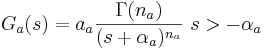
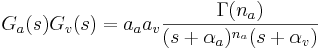
For this analysis, it is assumed that the auditory filter is a simple gammatone or gammachirp filter, without any compression built in. This means that the filter has a known envelope of the form  where the subscript a refers to the fact that this is the auditory filter. The terms of this equation are as follows: aa gives an overall amplitude, the
  gives a finite rise time and the
  gives the decay. The time that the maximum occurs can be found by differentiating the filter envelope, and is found to be at t = (na − 1) / αa. This envelope, with a sinusoidal carrier -- a gammatone filter -- can be seen in Figure 10. The envelope of the resonance of the vocal tract is taken to be a simple damped exponential:
  , with the v referring to the vocal tract filter. We assume that the entire system of vocal tract resonator followed by auditory filter is struck by a stream of pulses which are modelled as single delta-functions
  where the tp are the pulse times. This is clearly a simplistic model of the resonances of the vocal tract, since the vocal filter cannot have an instantaneous rise time, but it will suffice for the purposes of defining constraints on the response of the system.
To simulate the output of the cochlea to the auditory nerve, the output of the basilar membrane is half-wave rectified. In many models, there is also a low-pass filter applied to the signal which simulates the loss of phase-locking in the hair cells at high frequencies. Since the NAP is monopolar, lowpass filtering is equivalent to leaky integration of the signal. For a first treatment of the problem, the low-pass filtering will be put aside, and signals which have simply been half-wave rectified will be considered. This class of signal is known as the Neural Activity Pattern, or NAP. Once an initial version of the model has been developed, the effect of low-pass filtering can be considered again.
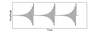
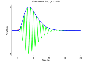
Single-pulse excitation
In the case of a single pulse exciting the filterbank, the response in a single channel is simply the impulse response shown above. This is the most simple form of excitation, and provides a good basis for developing an algorithm which will ultimately extract the timings and amplitudes of filtered pulses. Figure 11 shows a simulated NAP for the 1000Hz channel of a gammatone filterbank which has been struck by a single pulse at time t = 0. This input is received as a function of time by the strobe finding mechanism. In the ideal case, the mechanism will wait as the amplitude of successive peaks gradually rises, and then fire a strobe at the top of the highest peak in the NAP. This requires the system to look ahead a certain amount of time to determine if it is indeed dealing with a rising set of peaks due to a pulse. However, the rise time of the filter is known; for a gammatone filter with a given centre frequency, the peak of the filter envelope is at t = (na − 1) / αa after the pulse, as shown above. This means that a simple constraint can be placed on the strobing system: in each channel, the system should wait for a maximum of (na − 1) / αa to see if a higher peak occurs during that time. In the high frequency channels, this time is short, but as the channel centre frequency decreases, this `look-ahead' time becomes longer.
This rise time of the filter runs from a maximum of about 15.6ms for a gammatone filter at 50Hz, to 0.83ms for a gammatone filter at 5kHz. Thus, looking forward as far as the rise time of the lowest gammatone filter requires a maximum look-ahead of about 16ms. After this time, a firm decision can be made on whether an event occurred at a certain time.
Once a strobe has occurred and the filter response starts to fall, the system can simply `follow' the decaying envelope of the filter down. Any peaks at or below the envelope of the decaying filter's response at a certain time after the strobe can be ignored. This is the system used in the decaying threshold of previous strobe finding algorithms. The decay parameters of the filter are already known: the envelope decays from a maximum at t = (na − 1) / αa following a gamma envelope.
Pulse-resonance excitation
The case of pulse-resonance excitation is an extension of the filtered pulse case. In this version, the pulse is filtered first by a resonance, and then by the auditory filter. The form of the vocal tract filter is taken to be the same as that of a gammatone filter, but with different coefficients.
The form of the envelope of this filtered response can be derived by convolving the envelopes of the impulse responses of the auditory filter and the vocal tract filter. Merely convolving the envelopes to get the combined envelope holds only when the carrier frequency of both the vocal tract and auditory filters are the same, but the on-frequency response of the filter provides an upper bound on the envelope of the response, as shown in section \ref{carrier}.
This convolution can be achieved in the Laplace domain. The Laplace transform of the function is
and the transform of is just 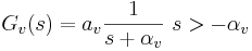
To perform a time domain convolution, the Laplace transforms of the two functions are simply multiplied to give
It is possible to calculate the inverse Laplace transform explicitly for certain numerical values of the constant na (the general solution is also possible, but it is not particularly useful in this case). na is difficult to generalise over, as it appears in the power in the denominator of the function in the Laplace domain. For the simple case of a damped exponential vocal tract resonance and a standard gammatone filter (na = 4) an explicit case of the general equation can be found. This is:

which has a similar form to the gamma envelope, but with exponents of both αa and αv and a polynomial in t rather than a single power of t.
This, then, is the form of the envelope of a gammatone auditory filter struck with a decaying exponential resonance. Formant bandwidths are of the order 50-125Hz (Hawks and Miller, 1995) for frequencies up to about 3kHz. The longest decay times will be associated with the smallest formant bandwidths, so for a 50Hz formant bandwidth, αv will be around  . This gives an upper bound on the expected envelope of the filter response when it is driven by a formant of speech. If the minimum formant bandwidth is taken as being 50Hz, then for a gammatone filter at 1000Hz, driven by a formant at 1000Hz with a 50Hz bandwidth, the rise time goes from about 4ms to about 7ms (4 cycles to 7 cycles). This maximum rise time can be calculated in each channel in the same way.
Adding a carrier
This analysis has so far been carried out only for the envelopes of the functions involved. If the carrier is included in the calculation as well, the ensuing expression becomes even more complicated. However, since we wish only to find upper and lower bounds on the decay time of the NAP peaks in response to a damped resonance, a simple heuristic analysis will suffice.
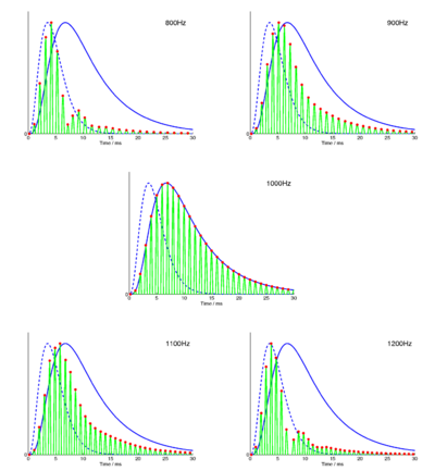
Figure 12 shows the effect of sweeping a damped formant through the filter with a centre frequency of 1000Hz. The formant has a frequency of 800, 900, 1000, 1100 and 1200 Hz in the five panels. The maximum temporal extent of the filter envelope is when it is driven exactly on frequency; the decaying resonance has the same carrier frequency as that of the channel of the filterbank which is being observed. In the off-frequency cases, the response of the filterbank will decay faster than in the on-frequency case, and will rise to its highest value faster. On-frequency excitation is the extremal case, both for the onset and the decay characteristics of the excited filter, and so the envelopes calculated above for a gammatone filter and a damped resonance are the limit of the expected response of the auditory filters when excited with damped resonances.
Multiple pulses
The system needs to be able to identify a series of pulses followed by resonances. If the pulse rate is high enough, new pulses will interfere with the tails of previous resonances. The interaction of a given resonance decay with the onset of the next pulse makes it somewhat more difficult both to identify pulses and to track the rise and fall of vocal tract resonances.
Noise excitation
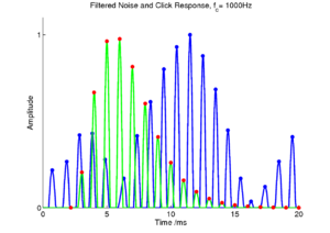
Another important input signal to consider is noise, as it can form part of a communication sound (for example fricatives in human speech) or be added to a signal which is to be retrieved. Figure 13 shows the effect of exciting one channel of a filterbank with Gaussian noise. Note that the output of the filter, when driven by a noise, is not necessarily at the same frequency as the filter's impulse response, and that the output frequency varies with time. In the case of bandpass filtered noise, there will be a general rise in the level of excitation for all filters in the region of the passband. A strobing system should degrade gracefully when processing any stimulus that is not a periodic, pulse-resonance signal. It should continue to issue strobes at a reasonable rate, but essentially at random. If there is no temporal structure to the input signal, then there will be no temporal structure in the SAI. In fact, the process of strobed temporal integration actively damps down noises in the SAI relative to pulse-resonance sounds. This happens because, in a noise, strobes will occur randomly, and the activity in each channel will tend to have a random phase. This means that the characteristic peaks and troughs in each SAI channel will become smeared out relative to the pattern for a pulse-resonance sound, and the overall level of activity in the SAI will be lower and the dynamic rage smaller than for a pulse-resonance sound. In this case, strobed temporal integration reverts to a form of spectrum analysis. The SAI for a noise will consist of sustained activity, proportional to the energy present in each channel.
The effect of low-pass filtering and compression
After the filterbank stage in AIM, the NAP stage simulates the response of the inner hair cells to the motion of the basilar membrane. The signal is first half-wave rectified to simulate the monopolar response of the hair cells. The loss of phase-locking at higher frequencies is then simulated with a low-pass filter, and since the signal has already been half-wave rectified at this point, this reduces to a simple leaky integrator. Loss of phase-locking is associated with the capacitance of the hair-cell synapse. The standard low-pass filter in AIM is a two-stage filter with a cutoff frequency of 1200Hz, meaning that the filter skirt is 24dB down by 4800Hz. For non-compressive filterbanks, such as the gammatone filter, compression is also added at this stage. For the gammatone, logarithmic compression is applied to the filter output before the rectification and filtering stages. To find the response of a driven filter, the envelope derived above can simply be processed in the same way as the output signal is.
A candidate system: Low-latency thresholding with constraints
Using the constraints described above, it is fairly simple to modify the parameters of some of the existing strobing systems to fulfil these constraints. A set of simple rules define the strobe system:
- All points which are not local maxima are ignored.
- When the signal exceeds threshold, the threshold is set to the level of the signal at that time, and that point is labelled as a strobe candidate.
- The threshold decays according to the longest possible decay of the filter in that channel when struck with a damped formant.
- If there are no larger strobe candidates within the rise time of the driven filter, then the candidate is labelled as a strobe.
To promote the propagation of strobes across multiple channels, an additional rule may be added:
- If a strobe is known to have occurred in a higher frequency channel, then the threshold in the current channel is lowered by a set proportion for each higher channel in which a strobe occurred. The threshold is lowered in a region around the time that a strobe is expected to occur.
In practice, this system modifies the thresholding functions from previous systems to include two filter-dependent parameters: the decay rate (and trajectory), and the `look-ahead' time, which is determined by the rise time of the filter. In practice this leads to a non-causal system, where there is a short delay in classifying strobe points. The parameters of the lower-frequency channels will determine the maximum values for the look-ahead time. If some maximum look-ahead is desired, then the look-ahead can be truncated in the low-frequency channels, at the expense of accuracy.
Time constants in each channel
For each channel of the filterbank, there are three parameters of interest in the response: these are the filter centre frequency (which determines the timing between NAP peaks), the maximum rise time of a driven filter (which determines the maximum look-ahead needed before classifying a strobe point), and the slowest decay rate of a driven filter (which determines the decay rate of the threshold). Given these parameters, the `temporal shadow' strobe criterion can be updated to take into account the known properties of the filter in each channel.
To determine the time constants in each channel, the filter response derived above is processed to mimic the effect of the NAP stage on the filter output. The filter envelope derived above is correct for a gammatone filterbank, and is low-pass filtered to simulate the NAP. The other filterbanks used in AIM, the PZFC and dcGC, do not have exactly the same impulse response as the gammatone, but to a first approximation the response is similar enough to allow for improved strobing. The compression applied by these filterbanks is less aggressive than the logarithmic compression used in the gammatone, so this stage can be left out when calculating the parameters of the envelope for these filterbanks. In practice, the parameters derived and used in the experiments below are for a low-pass filtered gammatone filter with no compression in all cases. The PZFC and dcGC filternbanks are described in detail in chapter 5; the methods and main results presented here are based on the use of the gammatone filterbank, but the experimental results also include values for the compressive dcGC and PZFC filterbanks for comparison purposes.
Once the envelope has been calculated, the maximum of the envelope can be found. The time to the maximum is the filter rise time. All the parameters for the strobing system can be pre-calculated once for a given set of filterbank parameters, and then reused. The parameters to be saved are the rise time, the filter centre frequency, and the form of the decaying threshold (this is used rather than a decay rate, since the absolute amplitude of the filter response will change on the basis of the input).
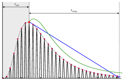
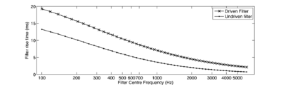
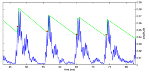
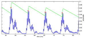
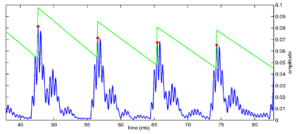
Figure 14 shows the envelope of a damped formant exciting a channel of a gammatone filter. The rise time trise is calculated in each channel. The system then waits for trise after each strobe candidate to see if any larger strobes occur in that time. If a larger NAP peak does occur, then the new peak is marked as a candidate. Once trise has passed since the first candidate, the last identified candidate is marked as the strobe point. Figure 15 shows the rise times for the channels of the standard gammatone filterbank when driven by an on-frequency formant.
There is a problem with such a simple lockout system. If the pulse-rate is faster than the lockout time, the system will not produce strobes on every pulse. To prevent the lockout from interfering with the pulse rate of the audio, a maximum lockout time can be set. This increases the chance of the system incorrectly identifying points on a rising edge in the low-frequency channels, but allows the system to strobe accurately on each peak of higher-pitched sounds. The maximum lockout is a configurable parameter. In testing it was found that good results are achieved when the strobe lockout is limited to a maximum of 6ms. This means that there is a maximum of 6ms delay between a NAP peak being identified, and being marked as a strobe point. It does, however, mean that the maximum rise time can be larger than the lockout for around two-thirds of the channels. In practice, this is not such a problem, since only a few channels will be driven strongly on-frequency at any given time. Looking at undriven filter rise times, we see that a 6ms rise time lockout only affects channels below about 450Hz. Furthermore, in the low-frequency channels there are few NAP peaks per pulse, and so the exact choice of NAP peak for strobing on is less important.
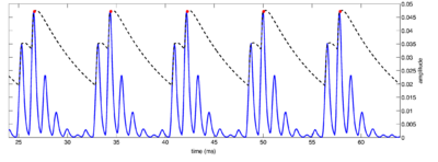
For simplicity, the temporal shadow strobe criterion (and all other previous strobe criteria) used a linearly decaying threshold from the highest NAP peak. This is simple to implement, but does not follow well the form of the actual filter decay. In initial testing of the new algorithm, it was found that strobing accuracy could be improved slightly by using a threshold that matches more closely the form of the driven filter envelope. Computationally, this approach is only slightly more expensive, but the increase is not significant because the form of the threshold in each channel can be pre-calculated and stored. Figure 16 shows the effect of applying the new constrained threshold in one channel of the filterbank. The threshold can be seen to rise a small amount before it falls. This occurs because the threshold is taken from being one NAP cycle (1/centre frequency) before the peak of the envelope, allowing for the case where the NAP peaks are out of phase with the envelope peak.
This new 'constrained thresholding' strobe detection has three major improvements over the older strobe detection systems. Firstly, all the parameters of the system are calculated from the derived envelopes of driven gammatone filters. These parameters provide an upper bound on the expected temporal characteristics of the filter response. Secondly, the 'lockout' system allows the system to follow a rising edge for a short period, and not issue a strobe point until the top of a rising edge. This means that the system will tend to issue strobe points on true local maxima of the filter envelope, rather than at the start of a rising edge (as the 'local maximum' criterion does). Finally, the form of the threshold in each channel is pre-calculated to follow the form of the decaying envelope of a driven filter in that channel. This threshold follows the real envelope of the NAP more closely than a linear threshold. The system, as described above, was implemented in AIM-MAT, and it is tested in the experiments below. Figure 17 shows the effect of running the system on a pulse train input with an 8ms interval between pulses.

A candidate system: Event-time back-projection
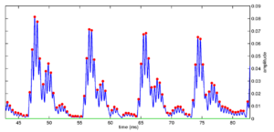
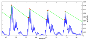
Given knowledge of the rise time and decay characteristics of the filter, it is possible to make an estimate of when an event occurred based on the amplitudes and timings of consecutive peaks of the NAP. This algorithm calculates a distance measure from the impulse response of the system to the current state at every point in time. This has the effect of tying together the responses of all channels and determining a single strobe time across the entire filterbank. The system marks the presence of a pulse in all channels, even if it is masked by other energy in some of those channels. To calculate strobes in this system, a summary statistic for the entire NAP is produced, by calculating a distance measure from the NAP at time t to the impulse response of the gammatone filterbank.
The impulse response of the filterbank is calculated for each channel. Then a summary statistic, the probability that the last section of the NAP was caused by a glottal pulse, is calculated. This summary probability is summed across channels to produce a single probability signal for the whole input, which represents the probability that the incoming signal was produced by a glottal pulse at that point. To calculate the probability, a pulse is first pre-processed through the filterbank, then the distance between the 'pulse NAP' and the current NAP state at each time is calculated. This summary signal is passed to the simple 'local maximum' decaying threshold strobe algorithm described earlier. The strobe points are then placed, based upon the known peaks in the impulse response of the filterbank for different channels. In this way it is possible to achieve continuous `strands' of strobe points across all channels. In this case, the strobe points are placed on the NAP peak closest to the detected strobe time.

Figure 18 shows the strobes generated by this back-projection algorithm for a small segment of a pulse train stimulus. The main notable feature of this system is that strobes always occur in all channels. The strobe position in each channel is set to be the NAP peak which is closest to the ideal strobe point in the 'pulse NAP'.
This approach is considerably more computationally expensive than a simple thresholding approach, since a section of the NAP must be compared against an entire saved impulse response for every time step. This increases the computational complexity of the system by several orders of magnitude. The system was implemented in AIM-MAT as described, but is not intended for use in a large-scale system. It is compared against the alternative systems below.
In preliminary testing of this system, the default parameters of the 'local maximum' strobe threshold (5ms lockout, 20ms decay time) were found to work well for all filterbanks apart from the PZFC. In the case of the PZFC, the dynamic range of the thresholded strobe probability signal was about half that of the other systems. In order to combat this effect, the decay time was extended to 50ms when using the PZFC with the back-projection strobe system.
The likely explanation for this behaviour is that the calculated impulse response of the PZFC filterbank does not match up well with the real impulse responses seen in the filterbank. The impulse response of the filterbank is calculated while the filterbank is in its initial state, before any adaptation has taken place. The 'cold' AGC in the PZFC will be in a different state to that when it has adapted to the incoming stimulus.
Testing strobe detection
Test stimuli
In order to test a strobe detection system, a set of stimuli with known pulse times is required. The effectiveness of the strobing system can then be measured with reference to the known pulse times of the original stimuli. Effectiveness can be assessed in terms of strobe rate or the precision of the predicted stimulus pulse times. Pulse trains and synthetic vowels were used to assess the effectiveness of the strobing systems.
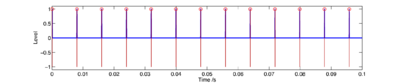
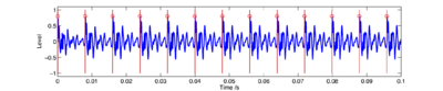
In the case of the click train and synthetic vowels, it is simple to ensure that the pulse times are known exactly. In the case of the real stimuli, it is possible to generate stimuli with known pulse times by first analysing the signal with STRAIGHT, and then re-synthesising with a known pitch track. Examples of the various synthetic stimuli and associated pulse times are shown in Figure 19 and Figure 20.
An added attraction of these stimuli is that they can easily be added together to create composite stimuli in order to test the effectiveness of strobing systems in multi-source environments, or even to test future systems that segregate stimuli on the basis of the source characteristics.
Methods
Using the synthetic stimuli detailed above, it is possible to test the various strobing systems on some basic criteria. We are interested in how many strobes there are in each channel for each pulse of the input sound, and what proportion of the pulses are correctly strobed upon. This gives a reasonable measure of how the strobe detection system is performing.
To test for the number of strobes per cycle in a single-source sound, a simple sliding window approach can be taken. The NAP and strobes are windowed into sections that are the width of the inter-pulse interval. Each section starts at the known pulse time, and the number of strobes in each section is counted. The system is deemed to be working correctly if there is exactly one strobe in each channel for each windowed section.
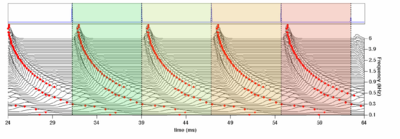
Figure 21 shows the windowed segments used by the single-source strobe detection system. If there is a one strobe per section in each channel, then the system is deemed to be working perfectly.
For multi-source sounds, this evaluation becomes slightly more complex, as the windows of interest are different for the different sources. In this case, the NAP and strobes are analysed sequentially. The pulse times are arranged in the order in which they occur (regardless of which source they came from). The system then iterates through the sequentially-ordered pulse-times, looking forward from the pulse time in each channel, and assigns the first strobe that it finds within the interval to that pulse. That strobe is then `claimed' by the strobe process, and cannot be used again. Once the complete sound has been processed, the system iterates over the remaining strobe points, and finds those intervals where there are unclaimed strobes. These intervals are marked as containing errors. This tests that the total number of strobes is roughly the same as the total number of pulses, and that the strobes occur at a reasonable rate. However, due to the slightly different methodology between the single-source and multi-source cases, the two sets of results cannot be compared directly.
Results
The following configurations of source stimulus were tested with various strobe algorithms and filterbanks:
- Single-rate pulse train
- Frequency-swept pulse train
- Synthetic vowel
- Two pulse trains with different rates
- Two synthetic vowels with different rates
For the single-source stimuli, all the available strobe algorithms were tested, including the 'constrained thresholding' and 'event time back-projection' schemes described above. For the two-source cases, the best-performing systems from the single-source tests were tested again. These were the 'local maximum' system and the two newly-developed systems.
Each of the algorithm variants is given a score from 0 to 100% on its ability to get the timing of the strobe points right, and the mean number of strobes per pulse is reported. This value is expected to be around 1 if the system is performing well.
Single-source stimuli
In the first experiment, a 200ms click train with 8ms between clicks was used as the input stimulus to a set of filterbanks and strobing algorithms. Each system was assessed with a percentage score for the proportion of windowed sections with exactly one strobe in each channel, and an overall number of strobes per pulse in each channel. <tablenameRef name="pulse_train_results"/> shows the results from this experiment.
| Algorithm | dcGC | PZFC | log(gammatone) | linear gammatone |
|---|---|---|---|---|
| peak | 13.8% | 9.1% | 9.9% | 10.1% |
| 6.82 | 9.92 | 10.1 | 9.47 | |
| temporal shadow | 56.4% | 24.1% | 9.0% | 12.2% |
| 1.40 | 1.82 | 3.65 | 2.17 | |
| local maximum | 95.6% | 92.9% | 89.5% | 94.2% |
| 0.96 | 0.93 | 1.02 | 0.98 | |
| constrained threshold | 95.9% | 93.7% | 92.7% | 95.6% |
| 0.97 | 0.94 | 1.00 | 0.97 | |
| back-projection | 90.3% | 84.6% | 92.0% | 88.9% |
| 0.92 | 1.00 | 0.92 | 0.92 | |
| parabola | 87.9% | 80.3% | 72.9% | 86.1% |
| 1.00 | 0.96 | 1.11 | 1.04 | |
| bunt | 89.3% | 85.8% | 59.5% | 81.5% |
| 0.94 | 0.90 | 1.01 | 0.91 | |
| lyon | 0.0% | 0.0% | 0.1% | 0.1% |
| 4.23 | 4.23 | 4.23 | 4.23 |
In the second experiment, the pulse train was swept in pulse interval from 10ms between pulses to 5ms between pulses. The total stimulus duration is 1 second. <tablenameRef name="swept_pulse_train_results"/> shows the results from this experiment.
| Algorithm | dcGC | PZFC | log(gammatone) | linear gammatone |
|---|---|---|---|---|
| peak | 14.3% | 9.2% | 10.4% | 10.4% |
| 6.43 | 9.14 | 9.9 | 9.07 | |
| temporal shadow | 63.7% | 32.6% | 11.5% | 15.2% |
| 1.36 | 1.77 | 3.62 | 2.10 | |
| local maximum | 98.9% | 96.8% | 94.3% | 98.2% |
| 1.00 | 0.97 | 1.05 | 1.00 | |
| constrained threshold | 93.4% | 92.3% | 91.4% | 93.1% |
| 0.94 | 0.93 | 0.99 | 0.95 | |
| back-projection | 94.9% | 95.4% | 96.8% | 91.7% |
| 0.99 | 1.00 | 1.00 | 0.99 | |
| parabola | 91.0% | 85.1% | 77.8% | 85.9% |
| 0.94 | 0.95 | 1.05 | 0.99 | |
| bunt | 89.5% | 88.0% | 60.7% | 83.1% |
| 0.94 | 0.92 | 1.01 | 0.91 | |
| lyon | 5.5% | 5.1% | 5.4% | 5.5% |
| 3.99 | 3.99 | 3.99 | 3.99 |
In the third experiment, a synthetic three-formant /a/ vowel was used. The stimulus duration was 200ms and the pulse interval was fixed at 8ms. <tablenameRef name="synthetic_vowel_results"/> shows the results from this experiment.
| Algorithm | dcGC | PZFC | log(gammatone) | linear gammatone |
|---|---|---|---|---|
| peak | 10.3% | 5.1% | 10.2% | 8.5% |
| 9.15 | 9.33 | 11.56 | 10.90 | |
| temporal shadow | 40.9% | 19.1% | 9.0% | 19.1% |
| 1.82 | 1.93 | 4.21 | 2.38 | |
| local maximum | 95.2% | 82.1% | 82.2% | 92.9% |
| 0.97 | 0.84 | 1.10 | 0.99 | |
| constrained threshold | 95.7% | 82.5% | 72.5% | 94.9% |
| 0.97 | 0.84 | 1.21 | 0.98 | |
| back-projection | 87.4% | 3.35% | 88.3% | 88.2% |
| 0.96 | 1.73 | 0.96 | 0.96 | |
| parabola | 85.5% | 72.7% | 66.9% | 76.2% |
| 1.03 | 0.93 | 1.18 | 1.16 | |
| bunt | 61.5% | 75.6% | 44.4% | 80.1% |
| 1.24 | 0.91 | 1.10 | 0.94 | |
| lyon | 0.0% | 0.0% | 0.1% | 0.1% |
| 4.23 | 4.23 | 4.23 | 4.23 |
Multi-source stimuli
The test system described above is less robust for the multi-source stimuli than it is for the single-source stimuli. For this reason, only those systems which were seen to perform particularly well with the single-source stimuli are assessed in this section. The three systems assessed are the 'local maximum' criterion and the new 'constrained threshold' and 'back-projection' systems. The results in this section are not directly comparable to the results for single-source stimuli, but these results do allow for basic comparison between algorithms.
The first stimulus is two pulse trains of the same amplitude, one with a repetition rate of 5ms and one with a repetition rate of 8ms. The total duration was 200ms. <tablenameRef name="two_pulse_train_results"/> shows the results from this experiment.
| Algorithm | dcGC | PZFC | log(gammatone) | linear gammatone |
|---|---|---|---|---|
| local maximum | 32.9% | 30.3% | 46.5% | 33.7% |
| 0.33 | 0.30 | 0.46 | 0.34 | |
| constrained threshold | 43.6% | 52.2% | 50.8% | 43.3% |
| 0.39 | 0.54 | 0.51 | 0.43 | |
| back-projection | 56.9% | 50.7% | 66.7% | 57.2% |
| 0.58 | 1.06 | 0.70 | 0.58 |
The second stimulus is two synthetic vowels, an /a/ vowel with an 8ms pulse rate and an /i/ vowel with a 5ms pulse rate. The two vowels had the same amplitude. <tablenameRef name="two_vowels_results"/> shows the results.
| Algorithm | dcGC | PZFC | log(gammatone) | linear gammatone |
|---|---|---|---|---|
| local maximum | 37.9% | 33.4% | 47.6% | 38.8% |
| 0.38 | 0.33 | 0.48 | 0.39 | |
| constrained threshold | 44.1% | 55.3% | 52.8% | 44.3% |
| 0.44 | 0.69 | 0.53 | 0.48 | |
| back-projection | 62.8% | 18.5% | 60.4% | 64.4% |
| 0.81 | 1.46 | 0.63 | 0.70 |
Discussion
The new constrained threshold and back-projection algorithms work well, both for single sources and combined sources. For single sources, the local maximum strobe criterion and the constrained threshold system exhibit very similar performance. This is, in many ways, unsurprising. It shows that the designers of the local maximum system were sensible in their choice of constraints, and used values which were already near optimal.
The performance of the local maximum and constrained threshold are comparable for single sources. For multiple sources, the constrained threshold system performs better (due to the faster decay rates in high-frequency channels) but the improvement is only very slight. The back-projection system works well (except in the case of the PZFC) and is much better than the others in the multi-source case. However, it remains a computationally expensive alternative. For the purposes of large-scale processing of datasets, computational load is a critical concern. As a rough benchmark, the constrained threshold strobe system takes about 10 seconds to process a 2 second noise in AIM-MAT on a 2.4GHz Intel Core 2 Processor. The back-projection system takes around 100 seconds to run on the same stimulus, so there is roughly an order of magnitude performance decrease associated with using back projection.
The back-projection system does not work well with the PZFC filterbank in all cases. As discussed above, it was necessary to increase the strobe threshold decay time for the thresholding system in the PZFC case because the dynamic range of the measured strobe probability was smaller than for the other filterbanks. Despite increasing the decay time, the back-projection system fails on the single-source vowel stimulus because the dynamic range is still too small. Further work to improve the performance of the PZFC with the back-projection strobe algorithm should be directed towards defining a 'canonical' filterbank impulse response from the PZFC, which can be compared with the impulse response in a range of AGC configurations. It is also the case that the zero-crossings of the PZFC shift with level in the current implementation. Replacing the current PZFC with a version where the zero-crossings do not shift with level may help aleviate the strobing problem.
The Lyon strobe detection system with a parabolic window performs very badly with respect to the criteria for a good strobe mechanism. The strobes-per-pulse values are identical for all filterbanks since the system has to produce a fixed number of strobes for a given stimulus length, and so performance can never be optimal. However, when this system was incorporated into the sound-effects recognition system described in chapter 6, it was found that performance with a SAI based on this system is actually slightly better than performance with a SAI which uses strobes from a simple thresholding based system. In this case, at least, is seems that optimal strobe detection is not such an important requirement.
Conclusions
Performance with the new strobe finding mechanisms based either on 'constrained thresholding' or 'event time back-projection' shows some slight improvements over previous systems. However, the change is not that great, and the 'local maximum' variant of the 'temporal shadow' strobe criterion performs almost as well as the new mechanisms in many cases. The default parameters for the temporal shadow criterion do not vary as a function of channel centre frequency, but they are similar to the parameters determined by the constraints described above for mid-range centre frequencies; the 5ms default strobe lag of the 'local maximum' system corresponds to the rise time of a driven filter at around 1600Hz, or an undriven filter at around 600Hz. The designers of previous strobe detection systems were careful to choose parameters which gave the best results possible, and succeeded in correctly identifying a good set of parameters for the dynamics of the filterbank they were using.
In this analysis, I have placed assumptions implicit in previous strobe detection systems on a firmer theoretical basis, and confirmed that the choice of constants made for these systems was reasonable. While the improvement gained by the 'constrained threshold' system described here over previous systems is small, the understanding of filterbank dynamics should prove useful for the development of future strobe detection systems.
An alternative strobe detection system was also introduced that compares the NAP to the impulse response of the filterbank at every time step. While this system is extremely effective at 'back-projecting' to find the original strobe time, it is inefficient and so cannot be used in a large-scale machine hearing system at this point in time. Further work would also be required to tune the parameters of this system in order to make it work correctly with the PZFC filterbank.
In the next chapter, the features developed in chapter 2 are computed from the stabilized auditory image, rather than from the cochleogram. We hypothesise that the stabilized features produced with strobed temporal integration will be more noise-robust than those generated from the NAP. The syllable recognition system developed in chapter 2 provides an excellent test-bed for the alternative features.
Bibliography
- Brown, G.J. and Cooke, M. (1994). “Computational auditory scene analysis.” Computer speech and language, 8, p.297-336. [1]
- Fant, G. (1960). Acoustic Theory of Speech Production. (Mouton De Gruyter, The Hague). [1]
- Hawks, J.W. and Miller, J.D. (1995). “A formant bandwidth estimation procedure for vowel synthesis.” J. Acoust. Soc. Am., 97, p.1343-1345. [1]
- Hess, W. (1983). Pitch determination of speech signals: algorithms and devices. (Springer-Verlag). [1] [2] [3] [4] [5] [6]
- Patterson, R.D. (1994). “The sound of a sinusoid: Spectral models.” J. Acoust. Soc. Am., 96, p.1409-1418. [1]
- Patterson, R.D. (1994). “The sound of a sinusoid: Time-interval models.” J. Acoust. Soc. Am., 96, p.1419-1428. [1]
- Robinson, K. and Patterson, R.D. (1995). “The stimulus duration required to identify vowels, their octave and their timbre.” J. Acoust. Soc. Am., 98, p.1858-1865. [1]